Statistical Arbitrage Through Cointegrated Stocks (Part 1): Engle-Granger and Johansen Cointegration Tests

Introduction

This is the first of two articles that demonstrate how to use cointegration in statistical arbitrage trading strategies. Statistical arbitrage trading strategies are mistakenly seen by many as magical zero-risk strategies on one side, and as practically impossible for the average retail trader on the other side. This misunderstanding is caused by legends created around astonishing results obtained by some big players, the eternal searching for the Holy Grail of trading by inexperienced people, and ultimately by the lack of knowledge about what statistical arbitrage is.

When properly developed and backed by the right order execution infrastructure, they can show low risk and consistent profitability in the long run. But, in general terms, they also require proper risk management as any other trading activity. Again, statistical arbitrage strategies are not magical zero-risk strategies.

In a previous article, we did a simple correlation-based pairs trading that performed well on the backtest, but failed miserably when we let it run for two weeks on a realtime demo account. Probably the most clear, textbook evidence that backtests are useful in assessing the viability of a strategy, but at the same time can say almost nothing about the real world. And more than that, clear evidence that statistical arbitrage is not risk-free. Even a promising strategy requires careful risk management, which we didn’t implement in our sample prototype, and an adequate order execution environment, which is the underlying subject in this article.

Why were the results so bad in the demo account when compared with the backtest? How could we improve our tools beyond the correlation coefficient that captures co-movement between two assets to have a more robust framework to detect long-term dynamics in more than two assets? How can we go beyond simple pairs trading and expand the portfolio to a group of stocks from the same sector?

Success on backtest, failure on realtime

Recently, my partner and I were in an informal meeting with a trader who is used to operating dollar contracts on the Brazilian Exchange B3. She said she would love to have the resources to try “some kind of stat arb on agricultural commodities”, but being a traditional discretionary trader trained in technical analysis and price action, without a strong background in math or statistics, she was positive in saying that statistical arbitrage would be “out of her reach”. She was echoing that well-known belief we talked about at the beginning, the belief that statistical arbitrage is not within the reach of the retail trader.

To make a long story short, and go right to what you are looking for here, we then turn that into a challenge among friends: what if we used our free time to develop an automated statistical arbitrage framework for learning purposes? But how to do that if none of us is a great statistician, mathematician, or has the computational power required to beat the big players? We did what learners usually do: we started doing academic research to understand the problem, the alternatives already found in the market, studying the successes, but also the failures.

Our first baby steps resulted in an article I published here recently about the mathematician and hedge fund manager Jim Simons and his legendary Medallion fund. In that article, we used a barebones EA to illustrate statistical arbitrage between XAUEUR and XAUUSD. 

The graph below shows our backtest results previously published here.

Fig. 1 - Backtest results from pairs-trading EA (previous article)

Then, to test its viability in the real world, we left that barebones EA running on a zero-spread commission-based demo account for two weeks. The results were catastrophic.

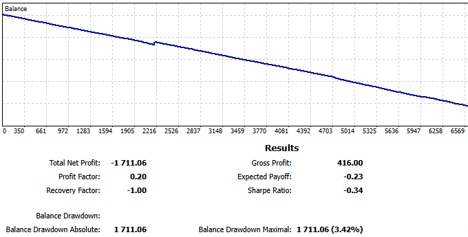
Fig. 2 - ReportHistory from two weeks on demo account for pairs-trading EA

Probable causes

When looking for the reasons for a failure in a trading strategy, we are tempted to start by “tweaking the parameters”. But let’s try a more systematic way, investigating the causes.

Two consecutive bad weeks?

Maybe it was simply two consecutive bad weeks on the market? Even on the backtest, we had some break-even periods and even some periods of minimal drawdown, don’t we?

Yes, but even in our worst weeks, we never had so many losses in sequence. In this realtime test, while our maximum consecutive wins were only four, our maximum consecutive losses amounted to forty-two! While our average consecutive wins were only one, our average consecutive losses were five. In summary, we were losing almost all trades!

Fig. 3 - sequence of losses from pairs-trading EA on demo account 

Obviously, there was something very wrong, something very different from our backtest environment. Moreover, because pairs trading is market-neutral by definition, meaning it is not tied to security returns.

"Pairs trading is a market-neutral investment strategy in its simplest form." [Gatev et al. 2006]

(Pairs trading, as the simplest form of statistical arbitrage, is generally, typically market-neutral. But our academic research shows that this is not always the case in a broad sense. There are situations where statistical arbitrage can carry market or sector risks, depending on the hedging method of choice. We will deal with this when working on the risk/money management module of our framework. For now, we can consider our simple pairs trading as market-neutral).

Jim Simons made lots of money while markets were imploding during the 2008 subprime crisis. The Medallion fund was not the only hedge fund to rely on statistical arbitrage. So why were they making millions while their peers were being dismembered by the crash? It seems like there is something that they were doing better than the competition. Despite the highly secretive nature of their operations, they left some precious clues that today are even obvious, but also frequently overlooked by retail traders. The Medallion team was, and still is, driven by huge amounts of high-quality data. Also, they invested in the best computational power and order routing speed.

So, a bad week probably is not the cause. It turns out that, although statistical arbitrage is market-neutral, it is at the same time very sensitive to data and timing.

New environment?

Maybe it was the change of broker, with a different spread? For pairs trading in very short-term operations with thousands of entries per week, the bid/ask spread could easily become a problem. As you know, the services offered by forex brokers are usually paid via bid/ask spread and/or percent-based commission billed over traded volume.

But we can discard the spread. For the backtest, I intentionally used a high spread account with ~170 pips on average for Gold and ~50 pips for XAUEUR. For the demo account, I changed to a raw spread, commission-based account charging ~20 pips on average for XAUUSD and ~10 pips for XAUEUR.

Since we had a lower bid/ask spread in the demo account, the spread is probably not the culprit here.

Slippage?

Arbitrage is usually sensitive to timing, and our pairs trading strategy is very sensitive to timing. So let’s see what our CFD broker Execution Policy agreement has to say about order timing.

“We execute most orders automatically, with minimal manual intervention. However, in volatile markets, execution may occur at a substantially different price from the quoted bid or offer or the last reported sale price at the time of order entry.”

The last one who comes to mind is the usual suspect: slippage. We were sending instant orders at market price, and someone was closing the gap first. If this is the case, nothing is wrong here. This kind of “frontrunning” is legitimate. It is, in fact, the name of the game in arbitrage. It only means someone has more and/or better resources: better hardware, collocated servers near the broker, or simply a better software optimized for high-performance, while we are using a prototype. Probably, we were losing the race for several players, each one with some of these advantages, and eventually some players with all the advantages. That is, some big players were humiliating our humble prototype. 

In the Metatrader 5 User Guide, we see that we can simulate delays on backtests. 

“Strategy tester enabled the emulation of network delays during an Expert Advisor operation in order to provide close-to-real conditions for testing. A certain time delay is inserted between placing a trade request and its execution in the strategy tester. From the moment of request sending till its execution the price can change. This allows users to evaluate how trade processing speed affects the trading results.

In the instant execution mode, users can additionally check the EA's response to a requote from the trade server. If the difference between requested and execution prices exceeds the deviation value specified in the order, the EA receives a requote.”

We did it by setting a random delay… 

Fig. 4 - Metatrader 5 Tester settings with simulated delay 

… and BINGO! Even if slippage is not the only culprit, our usual suspect seems to be the main suspect here.

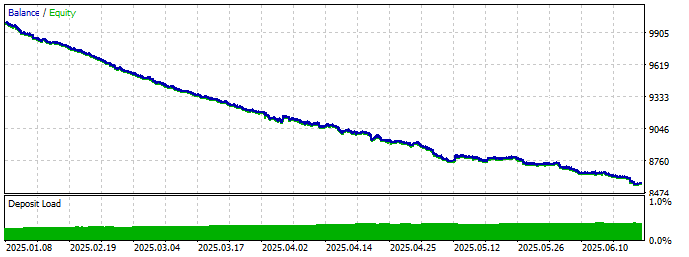
Fig. 5 - Resulting graph after running with simulated delay 

We could try to set the maximum allowed deviation in our code, but this restriction would undermine our strategy all. For it to be profitable, we need to catch the right price almost instantaneously. Besides that, normally, setting the maximum deviation is available only in professional accounts, which would take us away from our primary goal of developing a statistical arbitrage framework for the average retail trader.

The main problem: execution

Arbitrage can be used to make money by buying and selling anything, from toasters to tokens, from commodities to currencies, and everything in between. We can imagine that it started when people started exchanging goods, even before the use of money in the sense we understand it today. The concept is simple: if that hypothetical toaster is underpriced in marketplace A, maybe we can buy it there and sell it on marketplace B, where it is being sold at “the right price”. If the price difference is enough to cover the transaction costs, we can make a profit with minimal risk. 

The catch is that profit with minimal risk attracts people. The higher the risk-profit ratio, the larger the crowd. When we talk about arbitrage in financial markets involving commodities and currencies, the profits can be huge, and the number of people trying to buy the underpriced asset will be huge as well, with every player struggling to bid before their competitors. The need to be the first to bid - and have the order filled - eventually led to the development of the High-Frequency Trading (HFT) infrastructure, methods, and practice. As you probably know, HFT is not that easy, and it is not cheap.

The main problem here is that the average retail trader doesn’t have the resources required to beat the big players in speed. Even if we ignore the lack of a high-skilled team of statisticians and mathematicians backed by high computational power to develop the models, today we still need at least a collocation, a high-performance code, a broker capable of dispatching/routing the order in a few milliseconds…

The backtest results showed the theoretical viability of the strategy in a context of ideal order execution. That is, our orders were being executed instantly for any practical measures. No network delays, no broker server errors. 

It is easy to see that it is not for the average retail trader. As humble retail traders, if we want to benefit from arbitrage in financial markets, we will need to find alternatives beyond our naive prototype of pairs trading. We need to explore and find patterns and anomalies that are not so tied to speed.

From correlation to cointegration

Previously, we introduced the financial market as Jim Simons described it, that is, as an enigma in a continuous state of change. An enigma that requires permanent adaptation from operators to maximize the gains and minimize the losses. We built a minimal “portfolio” of two assets, XAUUSD and XAUEUR, and we chose the deviation from the mean of their quotation against the American dollar as the statistical relationship to look for. The widening of the spread and the posterior return to the mean were our entry and exit signals, respectively.

At this point, our statistical arbitrage “portfolio” is very limited, as are our statistical relationships. Moreover, because speed is out of our control, we can consider speed as a premature optimization for now. First, we must improve our capabilities before we spend our time on what is out of our control. We need to expand our portfolio. We need to have more statistical relationships in our screening arsenal and more statistical measures to be the trading trigger.

The criteria we used to select those pairs were correlation. We limited our search to the Forex majors and selected the most correlated pair in a given time interval. Now we will incorporate cointegration in our portfolio building selection.

According to statisticians, 

"Correlation captures only short-term relationships, while cointegration captures equilibrium relationships in the long run. Two variables can be highly correlated but not cointegrated, and vice versa." [Alexander, 2001]

The correlation coefficient tells us how much the prices of XAUUSD and XAUEUR tend to move in the same direction simultaneously. A cointegration test will detect an equivalence between the assets that is valid in the long term. Besides that, when using the correlation coefficient, we are limited to two assets, but when testing for cointegration, this limitation doesn’t apply, meaning that we can test several portfolio candidates at the same time. This makes a cointegration test ideal for our purposes here.

As traders or EA developers, we don't need to know the math behind cointegration tests. Since we will be using the Python Integration for Metatrader 5 for our data analysis and portfolio selection, we can use the ready-made Python functions from specialized libraries. Also, the AI assistants that I checked when writing this article - including the Metatrader 5 embedded GPTs - can help and save you time when developing simple scripts for this purpose.

As traders, we need to know what cointegration means and how we can use it to identify opportunities, particularly in the stock market, where cointegration is known to be more useful and effective than with currencies. As EA developers, we need to know how to use the best libraries available and how to interpret the results, so we can iterate and improve. By using high-quality libraries - and the Python ecosystem excels in mathematical, statistical, and machine learning high-quality libraries - we save time, avoid errors, and possibly have better performance.

If you want to go deeper into the topic, I would recommend that you take a look at the book quoted right above, from author Carol Alexander, more specifically, its chapter 12, which is entirely dedicated to cointegration. In that book, Ms. Alexander draws from the history of the use of cointegration in finance to its applicability in different markets, including Foreign Exchange (Forex). Her textbook is a very well-known reference in the field.

Let’s see how we can apply two of the most recommended cointegration tests, the Engle-Granger test and the Johansen test, in different asset classes and how to read their results.

The Engle-Granger cointegration test

The Engle-Granger cointegration test can be used to evaluate the level of cointegration between two assets. Its purpose is to answer the question: Do these two assets share a long-term equilibrium relationship? In what concerns us as traders and EA developers, this test will tell us if the two assets' spread is mean-reverting. But the answer is not binary, yes or no. Much like the Pearson Correlation Test we saw previously, it will return us a relative value (p-value) that should be put side-by-side with the results of other pairs to tell us which of them is the most integrated. 

The p-value is the probability of observing the data if there were NO cointegration. That is, the lesser the p-value, the better. There are well-known thresholds. A p-value < 0.05 is usually taken as a moderate signal of cointegration. A p-value < 0.01 is a strong signal, and any p-value > 0.05 is a signal of no cointegration. As always in trading, you should fine-tune these thresholds for your specific use case.

The Python code to perform both cointegration tests uses the well-known statsmodels library. 

“a Python module that provides classes and functions for the estimation of many different statistical models, as well as for conducting statistical tests, and statistical data exploration.”

from datetime import datetime, timedelta
import MetaTrader5 as mt5
import pandas as pd
import numpy as np
from statsmodels.tsa.stattools import coint
import matplotlib.pyplot as plt

# connect to MetaTrader 5 terminal
if not mt5.initialize(login=********, server="MetaQuotes-Demo",password="********"):
    print("initialize() failed, error code =",mt5.last_error())
    quit()

# Forex majors - check your Market Watch names
symbols = ['EURUSD', 'GBPUSD', 'USDJPY', 'AUDUSD', 'USDCAD', 'NZDUSD', 'USDCHF']

We are looking for the most cointegrated pair among the forex majors. We are not expecting to find a high cointegration rate. It will only serve as an illustration of how the Engle-Granger test works.

# define the timeframe and the number of days
timeframe = mt5.TIMEFRAME_D1  # Daily
n_days = 600
utc_to = datetime.now()
utc_from = utc_to - timedelta(days=n_days)

We will use the utc_from and utc_to variables to request symbol quotes with mt5.copy_rates_range for 600 trading days. One year has approximately 250 trading days.

# download historical data for each symbol
data = {}

for symbol in symbols:
    # Make sure the symbol is available in Market Watch
    mt5.symbol_select(symbol, True)
    
    # Get historical rates
    rates = mt5.copy_rates_range(symbol, timeframe, utc_from, utc_to)
    
    if rates is None or len(rates) == 0:
        print(f"No data for {symbol}.")
        continue

    df = pd.DataFrame(rates)
    df['time'] = pd.to_datetime(df['time'], unit='s')
    df.set_index('time', inplace=True)
    data[symbol] = df['close']

In this for loop, we request the closing quotes for each symbol, convert them to a Pandas DataFrame, and set the ‘time’ array as our tabular data index.

After concatenating the data frames and removing lines with missing values that could distort our results, we run the cointegration test.

# Store cointegration test results
results = []

# Test all unique pairwise combinations for cointegration
pairs = [(a, b) for i, a in enumerate(data.columns) for j, b in enumerate(data.columns) if i < j]

print("Cointegration test results (Engle-Granger):")
for a, b in pairs:
    score, pvalue, _ = coint(data[a], data[b])
    results.append((a, b, pvalue))
    print(f"{a} vs {b} | p-value: {pvalue:.4f}")

Index(['EURUSD', 'GBPUSD', 'USDJPY', 'AUDUSD', 'USDCAD', 'NZDUSD', 'USDCHF'], dtype='object')
Cointegration test results (Engle-Granger):

EURUSD vs GBPUSD | p-value: 0.3183
EURUSD vs USDJPY | p-value: 0.6990
EURUSD vs AUDUSD | p-value: 0.9308
EURUSD vs USDCAD | p-value: 0.9206
EURUSD vs NZDUSD | p-value: 0.9741
EURUSD vs USDCHF | p-value: 0.4342
GBPUSD vs USDJPY | p-value: 0.3273
GBPUSD vs AUDUSD | p-value: 0.7995
GBPUSD vs USDCAD | p-value: 0.6264
GBPUSD vs NZDUSD | p-value: 0.7810
GBPUSD vs USDCHF | p-value: 0.0238
USDJPY vs AUDUSD | p-value: 0.6299
USDJPY vs USDCAD | p-value: 0.5620
USDJPY vs NZDUSD | p-value: 0.6398
USDJPY vs USDCHF | p-value: 0.2377
AUDUSD vs USDCAD | p-value: 0.1260
AUDUSD vs NZDUSD | p-value: 0.2920
AUDUSD vs USDCHF | p-value: 0.5980
USDCAD vs NZDUSD | p-value: 0.0052
USDCAD vs USDCHF | p-value: 0.8574
NZDUSD vs USDCHF | p-value: 0.6384

Most cointegrated pair: USDCAD and NZDUSD (p = 0.0052)

Once we have the two most cointegrated pairs, we can decide if we incorporate them into our pairs trading portfolio. In the plot below, we can see clearly that the spread is returning to the mean, but the question is: is it worth the trade?

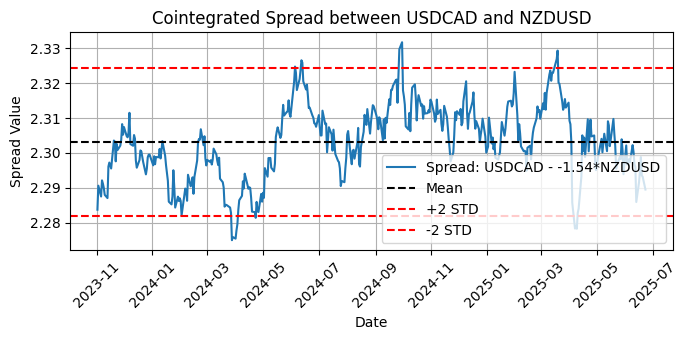
Fig. 6 - Plot of the cointegrated  spread between USDCAD and NZDUSD with mean and two standard deviations

The dashed black line indicates the mean of the spread. This is the long-term equilibrium level. The two dashed red lines indicate the two standard deviation (STD) bands. These define thresholds for identifying possible trading signals when the spread is unusually high or low, so the number of standard deviations is a serious candidate for your optimization. 

The hedge ratio

Note the -1.54 value used in the calculation of the long-term spread.

Spread = USDCAD - (-1.54) * NZDUSD

or

USDCAD + 1.54 * NZDUSD

This value is the hedge ratio. This is the optimal ratio, statistically estimated via linear regression, that aligns USDCAD and NZDUSD so that their spread is stationary, that is, it oscillates around the constant mean, which is key to mean-reversion strategies. By using this hedge ratio, we know we are comparing prices on the same scale, correcting for their volatility and directional relationship.

The spread captures the relative mispricings. In pairs trading parlance, we would say that when the spread is above +2 STD, it is historically high and we can consider shorting the spread; conversely, when the spread is below -2 STD, it is historically low and we can consider buying the spread.

To construct a market-neutral pair for trading based on this data, for each unit of USDCAD that we would go long, we would simultaneously go short 1.54 units of NZDUSD (or vice versa, depending on the signal direction). Then, when the spread reverts toward the mean, we exit the trade, closing both positions.

You can use this same code with symbols from any market or asset class. To use it as is, just replace the symbol names right on top.

The Johansen cointegration test

The Johansen cointegration test aims to answer the same question as the Engle-Granger test: do these assets share a long-term equilibrium relationship? In practice, and for our purposes here, the main difference is that the Johansen test can evaluate more than two assets at the same time and will tell us if these N assets share a common mean-reverting spread. We can think of it as a powerful tool to evaluate the possible cointegration in a group of stocks from the same sector, like oil stocks, tech stocks, etc. It allows us to find three, four, or more stocks (or any asset for that matter) that share a common long-term equilibrium relationship.

It checks whether there are combinations of the variables that are mean-reverting (stationary), even if the original series are not, and estimates how many cointegrating relationships exist between the variables. This number is called the cointegration rank.

The test produces two main statistics: the Trace Statistic and the Critical Value.

You get one trace statistic for each possible rank (0, 1, 2, ..., N−1 where N is the number of series). A larger trace statistic suggests stronger evidence of cointegration. The Critical Value is the threshold against which the trace statistic is compared. It depends on:

• The number of variables being evaluated
• The length of the sample
• The confidence level (90%, 95% or 99%)

In this specific case, we can think of the number of variables as the number of symbols being tested.

# Johansen Test
from datetime import datetime, timedelta
import MetaTrader5 as mt5
import pandas as pd
import numpy as np
from statsmodels.tsa.stattools import coint
from statsmodels.tsa.vector_ar.vecm import coint_johansen
import matplotlib.pyplot as plt
# Create a matrix for the test
log_prices = data.apply(np.log)

johansen_result = coint_johansen(log_prices, det_order=0, k_ar_diff=1)

# Trace statistics and critical values
print("\nJohansen Test Results (Trace Statistic):")
for i, stat in enumerate(johansen_result.lr1):
    cv = johansen_result.cvt[i, 1]  # 5% critical value
    print(f"Rank {i}: Trace Stat = {stat:.2f} | 5% CV = {cv:.2f} | {'Significant' if stat > cv else 'Not significant'}")

We can see the results for the other confidence levels by setting:
johansen_result.cvt[i, 0] for 90%
johansen_result.cvt[i, 2] for 99%

For the 95% confidence level (5% critical value), these are our results for the Forex majors in the same period and D1 timeframe we tested with Engle-Granger.

Index(['EURUSD', 'GBPUSD', 'USDJPY', 'AUDUSD', 'USDCAD', 'NZDUSD', 'USDCHF'], dtype='object')

Johansen Test Results (Trace Statistic):

Rank 0: Trace Stat = 105.25 | 5% CV = 125.62 | Not significant
Rank 1: Trace Stat = 68.10 | 5% CV = 95.75 | Not significant
Rank 2: Trace Stat = 42.01 | 5% CV = 69.82 | Not significant
Rank 3: Trace Stat = 25.83 | 5% CV = 47.85 | Not significant
Rank 4: Trace Stat = 11.73 | 5% CV = 29.80 | Not significant
Rank 5: Trace Stat = 5.74 | 5% CV = 15.49 | Not significant
Rank 6: Trace Stat = 0.58 | 5% CV = 3.84 | Not significant

As was expected, we have no significant cointegration among the seven Forex majors.

But if we test the two well-known Google and Nvidia stocks in the H1 timeframe (see below), we have a significant cointegration result for the same period and confidence interval.

Index(['NVDA', 'GOOGL'], dtype='object')
Number of observations: 5769
Number of variables: 2

Johansen Test Results (Trace Statistic):
Rank 0: Trace Stat = 18.71 | 5% CV = 15.49 | Significant
Rank 1: Trace Stat = 0.29 | 5% CV = 3.84 | Not significant

Most cointegrated pair (Engle-Granger): NVDA and GOOGL | p-value: 0.0824

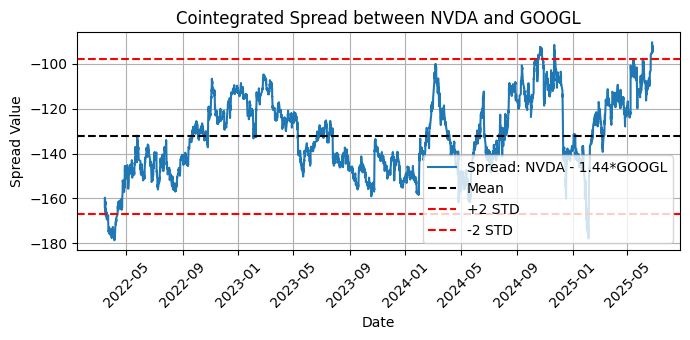
Fig. 7 - Plot of the cointegrated  spread between NVDA and GOOGL with mean and two standard deviations

Ok, we have significant cointegration for GOOGL and NVDA according to Johansen, but an Engle-Granger p-value above 0.05, which is a signal of no cointegration. Why these contradictory results? What does this mean?

Let’s run the same script with only the order of the symbols reversed, and you’ll see one interesting difference between the Engle-Granger and Johansen tests.

Index(['GOOGL', 'NVDA'], dtype='object')
Number of observations: 5769
Number of variables: 2

Johansen Test Results (Trace Statistic):
Rank 0: Trace Stat = 18.71 | 5% CV = 15.49 | Significant
Rank 1: Trace Stat = 0.29 | 5% CV = 3.84 | Not significant

Most cointegrated pair (Engle-Granger): GOOGL and NVDA | p-value: 0.0403

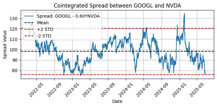
Fig. 8 - Plot of the cointegrated  spread between GOOGL and NVDA with mean and two standard deviations

As you can see, the Engle-Granger is sensitive to the order, while Johansen was not affected by the change. If you go deep into the Johansen test subtleties, you’ll learn that it can show some sensitivity to order in some cases, in particular for short samples or if we are at the edge of statistical significance. But as a general rule, it is theoretically insensitive to the order. If you find it returning inconsistent results after order changing, try adding more data to your sample as a first measure. This is why we replaced the D1 (daily) timeframe with an H1 (hourly) timeframe, to provide a bigger sample to the test.

Knowing that Engle-Granger is sensitive to the order of the variables suggests that you should always test both directions and assess the results by visual inspection of the plots to see if the spread is returning to the mean

Testing the stationarity of the spread

The spread is a time series, and to be sure it is returning to the mean, we need to check for its stationarity, that is, we need to check if its mean, variance, and covariance don't change over time. It is easier to model and forecast using techniques like ARIMA models if the time series is stationary.

The same Python library we have been using to test for cointegration has ready-made functions to test for stationarity, the Augmented Dickey Fuller (“ADF”) test, and the Kwiatkowski-Phillips-Schmidt-Shin (“KPSS”) test.

from statsmodels.tsa.stattools import adfuller

(...)

adf_result = adfuller(spread)

ADF Test on Spread:
 ADF Statistic : -3.0946
 p-value         : 0.0270
 Critical Values:
    1%: -3.4315
    5%: -2.8620
    10%: -2.5670

✅ The spread is stationary (reject the null hypothesis).

from statsmodels.tsa.stattools import kpss

(...)

def run_kpss(series, regression='c'):
    statistic, p_value, lags, crit_values = kpss(series, regression=regression, nlags='auto')

(...)

# Run KPSS test on the residuals
run_kpss(spread, regression='c')  # 'c' = test for level stationarity (use 'ct' for trend)

KPSS Test on Spread:
 KPSS Statistic : 2.2702
 p-value          : 0.0100
 Lags Used      : 44
 Critical Values:     10% : 0.347
    5% : 0.463
    2.5% : 0.574
    1% : 0.739

❌ The spread is NOT stationary (reject null of stationarity).

It seems like we have contradictory results again. ADF is saying that our spread is stationary, but KPSS doesn’t agree. Don’t panic. The statsmodels maintainers were careful enough to provide us with a clear explanation on how to interpret both tests in any possible combination of results. Here I’ll quote the statsmodels doc because I think it is hard to be more concise and clear.

“Case 1: Both tests conclude that the series is not stationary - The series is not stationary

Case 2: Both tests conclude that the series is stationary - The series is stationary

Case 3: KPSS indicates stationarity and ADF indicates non-stationarity - The series is trend stationary. Trend needs to be removed to make the series strict stationary. The detrended series is checked for stationarity.

Case 4: KPSS indicates non-stationarity and ADF indicates stationarity - The series is difference stationary. Differencing is to be used to make series stationary. The differenced series is checked for stationarity.”

So now we are informed that our spread is difference stationary and not strict stationary. What does this mean? It means that this time series may drift, but the changes are stable. It can be transformed into a strict stationary time series by simply taking the differences between consecutive values. Not surprisingly, this technique is called differencing. It removes trends and seasonality and makes our time series ready for more effective analysis and forecasting.

Do we need to make our spread a strict stationary? Many time series models require the data to be stationary, but this is not our case. We will not deal with forecasting models in our cointegration implementation. 

We will not run forecasting at all, but maybe it does no harm to know that the cointegration analysis doesn’t end with the cointegration tests.

Conclusion

In this article, we went one step further in the building of our statistical arbitrage framework for the humble retail trader. We added two more tools to our portfolio building statistical toolkit, the Engle-Granger and the Johansen cointegration tests. We saw what to expect from each of them and how to do the most basic interpretation of their results. Also, we saw how to check the stationarity of the spread using the Augmented Dickey Fuller (“ADF”) test and the Kwiatkowski-Phillips-Schmidt-Shin (“KPSS”) test.

This was the first of two articles introducing the basic tools. The following article will complement this primer with an implementation, backtests, and optimizations for a pair of cointegrated forex symbols and for a group of cointegrated stock symbols from the same sector.

I dare to say that the most relevant content here is not the presentation of the tools, the functions, or even the sample code. The most relevant piece of knowledge here is that if you are a retail trader, not a mathematical or statistics inclined person, a non-developer trader, the most valued skill you have when developing your statistical arbitrage strategy is the understanding of the asset or group of assets you work with.

Your knowledge about the markets is priceless, because the hard work in mathematics and statistics was already done for you by high-skilled professionals, and this work is available for free in many open-source libraries, including MQL5 libraries available on the Metatrader 5 platform along with the invaluable AI Assistant to help you with the proper implementation. 

Lesson learned: if you have limited resources, stay away from speed-dependent strategies and try to explore the data in creative ways, leveraging your market knowledge. 

References

• Alexander, C. (2001). Market Models: A Guide to Financial Data Analysis, Wiley.
• Engle, R. F., & Granger, C. W. J. (1987). Co-integration and error correction: representation, estimation, and testing. Econometrica.
• Gatev, E., Goetzmann, W. N., & Rouwenhorst, K. G. (2006). "Pairs Trading: Performance of a Relative-Value Arbitrage Rule." Review of Financial Studies.
• Johansen, S. (1988). Statistical analysis of cointegration vectors. Journal of Economic Dynamics and Control.

Attached file	Description
coint.ipynb	This file is a simplified Jupyter notebook containing Python code to run a single Engle-Granger cointegration test for a pair of trading instruments.
coint_googl_nvda.ipynb	This file is a extended Jupyter notebook containing Python code to run both the Engle-Granger and the Johansen cointegration tests over a (theoritically) unlimited number of trading instruments, along with the test for spread stationarity.
helper_quotes_to_db.ipynb	This file is a helper to save downloaded symbol quotes to an sqlite3 database. It is also a Jupyter notebook with Python code. Its purpose is to avoid redundant downloads and make possible to work offline.