MQL5 Wizard Techniques you should know (Part 07): Dendrograms

Introduction

This article which is part of a series on using the MQL5 wizard looks at dendrograms. We have considered already a few ideas that can be useful to traders via the MQL5 wizard like: Linear discriminant analysis, Markov chains, Fourier transform, and a few others, and this article aims to take this endeavor further of looking at ways of capitalizing on the extensive ALGLIB code as translated by MetaQuotes together with the use of the inbuilt MQL5 wizard, to proficiently test and develop new ideas.

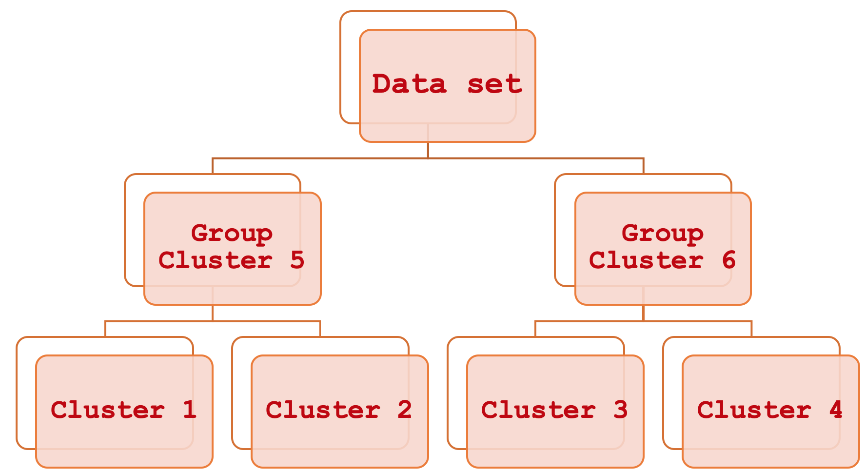
Agglomerative Hierarchical Classification sounds like a mouthful but it’s actually quite simple. Put plainly it is a means of relating different parts of a dataset by first considering the basic individual clusters and then systematically grouping them a step at a time until the entire dataset can be viewed as a single sorted unit. The output of this process is a hierarchical diagram more commonly referred to as a Dendrogram.

This article will focus on how these constituent clusters can be used in assessing and thus forecasting price bar range but unlike in the past where we did this to help in trailing stop adjustment, we will consider it here for money management or position sizing purposes. The style to be adopted for this article will assume the reader is relatively new to the MetaTrader platform and MQL5 programming language and as such we may dwell on some topics and areas that are jejune for more experienced traders.

The importance of accurate price range forecasts is largely subjective. This is because its significance mostly depends on the trader’s strategy and overall trade approach. When would it not matter much? Well this could be, in situations for example; if in your trade-setups firstly you engage minimal to no leverage, you have a definitive stop loss, and you tend to hold positions over extended periods which could run into say months, and you have fixed margin position sizing (or even a fixed lot approach). In this case price bar volatility can be put on a backburner while you focus on screening for entry and exit signals. If on the other hand you are an intra-day trader, or someone who employs a significant amount of leverage, or somebody who does not hold trade positions over weekends, or anybody with a mid to short horizon when it comes to exposure to the markets then price bar range is certainly something you should pay attention to. We look at how this can be of use in money management by creating a custom instance of the ‘ExpertMoney’ class but applications of this could spread beyond money management and even encompass risk, if you consider that the ability to understand and reasonably forecast price bar range could help in deciding when to add on to open positions and conversely when to reduce.

Volatility

Price bar ranges (which is how we quantify volatility for this article) in the context of trading are the difference between the high and low of a traded symbol’s price within a set timeframe. So, if we take say the daily time frame, and in a day the price for a traded symbol rises as high as H and not above H and falls as low as L and again not below L then our range, for the purposes of this article, is:

H – L;

Paying attention to volatility is arguably significant because of what is often called volatility clustering. This is the phenomenon of high volatility periods tending to be followed by more volatility and conversely low volatility periods also being followed by lower volatility. The significance if this is subjective as highlighted above however for most traders (including all beginners in my opinion) knowing how to trade with leverage can be a plus in the long run, since as most traders are familiar that high bouts of volatility can stop-out accounts not because the entry signal was wrong but because there was too much volatility. And most would also appreciate that even if you had a decent stop loss on your position there are times when the stop loss price may not be available, take the swiss franc debacle of January 2015, in which case your position would get closed by the broker at the next best available price which is often worse than your stop loss. This is because only limit orders guarantee price, stop orders and stop losses do not.

So, price bar ranges besides providing an overall sense of the market environment, can help in guiding on entry and even exit price levels as well. Again, depending on your strategy, if for instance you’re long a particular symbol, then the extents of your price bar range outlook (what you’re forecasting) can easily determine or at least guide where you place your entry price and even take profit.

At the risk of sounding mundane, it may be helpful to highlight some of the very basic price candle types and also illustrating their respective ranges. The more prominent types are the bearish, bullish, hammer, gravestone, long-legged, and dragonfly. There are certainly more types but arguably these do cover what one would most likely encounter when faced with a price chart. In all these instances as shown in the diagrams below, the price bar range is simply the high price less the low price.

Agglomerative Hierarchical Classification

Agglomerative Hierarchical Classification (AHC) is a method of classifying data into a preset number of clusters and then relating these clusters in a systematic hierarchical manner through what is called a dendrogram. The benefits of this mostly stem from the fact that the data being classified is often multi-dimensional and therefore the need to consider the many variables within a single data point is something which may not be too easy for one to grapple with when making comparisons. For example, a company looking to grade its customers based on the information they have from them could utilize this since this information is bound to be covering different aspects of the customers’ lives such as past spending habits, their age, gender, address, etc. AHC, by quantifying all these variables for each customer creates clusters from the apparent centroids of each data point. But more than that these clusters get grouped into a hierarchy for systematic relations so if a classification called for say 5 clusters then AHC would provide in a sorted format those 5 clusters meaning you can infer which clusters are more alike and which are more different. This cluster comparison though secondary can come in handy if you need to compare more than one data point and it turns out they are in separate clusters. The cluster ranking would inform how far apart the two points differ by using the separation magnitude between their respective clusters.

The classification by AHC is unsupervised meaning it can be used in forecasting under different classifiers. In our case we are forecasting price bar ranges, someone else with the same trained clusters could use them to forecast close price changes, or another aspect pertinent to his trading. This allows more flexibility than if it was supervised and trained on a specific classifier because in that instance the model would only be used to make forecasts in what it was classified, implying forecasting for another purpose would require retraining a model with that new data set.

Tools and Libraries

The MQL5 platform, with the help of its IDE, does allow as one would expect developing custom expert advisors from scratch and in order to showcase what is being shared here we could take that route hypothetically. However, that option would involve making a lot of decisions regarding the trading system that could have been taken differently by another trader when faced with implementing the same concept. And also, the code of such an implementation could be too customized and may be error- prone to be easily modified for different situations. That is why assembling our idea as part of other ‘standard’ Expert advisor classes provided by the MQL5 wizard is a compelling case. Not only do we have to do less debugging (there are occasional bugs even in MQL5’s in built classes but not a lot), but by saving it as an instance of one the standard classes, it can be used and combined with the wide variety of other classes in the MQL5 wizard to come up with different expert advisors which provides a more comprehensive test-bed.

MQL5 library code provides classes of AlgLib, which have been referenced in earlier articles in these series, and will be used again for this article. Specifically, within the ‘DATAANALYSIS.MQH’ file we will rely on ‘CClustering’ class and a couple of other related classes in coming up with an AHC classification for our price series data. Since our primary interest is price bar range it follows that our training data will consist of such ranges from previous periods. When using data training classes from the data analysis include file typically this data is placed in an ‘XY’ matrix with the X standing for the independent variables, and the Y representing the classifiers or the ‘labels’ to which the model is trained. Both are usually furnished in the same matrix.

Preparing Training Data

For this article though, since we are having unsupervised training, our input data consists only of the X independent variables. These will be historical price bar ranges. At the same time though we would like to make forecasts by considering another stream of related data that is the eventual price bar range. This would be equivalent to the Y mentioned just above. In order to marry these two data sets while maintaining the unsupervised learning flexibility we can adopt the data struct below:

//+------------------------------------------------------------------+
//|                                                                  |
//+------------------------------------------------------------------+
class CMoneyAHC                  : public CExpertMoney
  {
protected:
   
   double                        m_decrease_factor;
   
   int                           m_clusters;                            // clusters
   int                           m_training_points;                     // training points
   int                           m_point_featues;                       // point featues


...


public:
                                 CMoneyAHC(void);
                                 ~CMoneyAHC(void);
                                 
   virtual bool                  ValidationSettings(void);
   //---
   virtual double                CheckOpenLong(double price,double sl);
   virtual double                CheckOpenShort(double price,double sl);
   //---
   void                          DecreaseFactor(double decrease_factor) { m_decrease_factor=decrease_factor;            }
   
   void                          Clusters(int value)                    { m_clusters=value;                             }
   void                          TrainingPoints(int value)              { m_training_points=value;                      }
   void                          PointFeatures(int value)               { m_point_featues=value;                        }

protected:

   double                        Optimize(double lots);
   
      
   double                        GetOutput();

   CClusterizerState             m_state;
   
   CAHCReport                    m_report;
   
   struct                        Sdata
                                 {
                                    CMatrixDouble  x;
                                    CRowDouble     y;
                                    
                                                   Sdata(){};
                                                   ~Sdata(){};
                                 };
                                 
   Sdata                         m_data;
   
   CClustering                   m_clustering;
   
   CRowInt                       m_clustering_index;
   CRowInt                       m_clustering_z;
      
  };

So, the historical price bar ranges will be collected as a fresh batch on each new bar. Experts generated by the MQL5 wizard tend to execute trade decisions on each new bar and for our testing purposes this is sufficient. There are indeed alternative approaches such as getting a large batch spanning many months or even years and then from testing examining how well the clusters of the model can separate eventual low volatility price bars from high volatility bars. Also keep in mind that we are using only 3 clusters where one extreme cluster would be for very volatile bars, one for very low volatility, and one for mid-range volatility. Again, one could investigate with 5 clusters for instance but the principle, for our purposes, would be the same. Place the clusters in order of most eventual volatility to least eventual volatility order and identify in which cluster our current data point lies.

Filling Data

The code for getting the latest bar ranges on each new bar and populating our custom struct will be as follows:

      m_data.x.Resize(m_training_points,m_point_featues);
      m_data.y.Resize(m_training_points-1);
      
      m_high.Refresh(-1);
      m_low.Refresh(-1);
      
      for(int i=0;i<m_training_points;i++)
      {
         for(int ii=0;ii<m_point_featues;ii++)
         {
            m_data.x.Set(i,ii,m_high.GetData(StartIndex()+ii+i)-m_low.GetData(StartIndex()+ii+i));
         }
      }

The number of training points define how large our training data set is. This is a customizable input parameter and so the data point features parameter. This parameter though defines the number of ‘dimensions’ each data point has. So, in our case we have 4 by default but this simply means we are using the last 4 price bar ranges to define any given data point. It is akin to a vector.

Generating Clusters

So, once we have data in our custom struct, the next step is to model it with the AlgLib AHC model generator. This model is referred to as a ‘state’ in the code listing and to that end our model is named ‘m_state’. This is a two-step process. First, we have to generate model points based on the provided training data and then we run the AHC generator. Setting the points can be thought of as initializing the model and ensuring all key parameters are well defined. This is called as follows in our code:

m_clustering.ClusterizerSetPoints(m_state, m_data.x, m_training_points, m_point_featues, 20);

The second important step is running the model to define the clusters of each of the provided data points within the training data set. This is done through calling the ‘ClusterizerRunAHC’ function as listed below:

m_clustering.ClusterizerRunAHC(m_state, m_report);

From the AlgLib end this is the meat and potatoes of generating the clusters we need. This function does some brief pre-processing and then calls the protected (private) function ‘ClusterizerRunAHCInternal’ which does the heavy lifting. All this source is in your ‘include\math\AlgLib\dataanalysis.mqh’ file visible from line: 22463. What could be noteworthy here is the generation of the dendrogram in the ‘cidx’ output array. This array cleverly condenses a lot of cluster information in a single array. Just prior to this a distance matrix will need to be generated for all the training data points by utilizing their centroids. The mapping of distance matrix values to cluster indices is captured by this array with the first values up to the total number of training points represent the cluster of each point with subsequent indices representing the merging of these clusters to form the dendrogram.

Equally noteworthy perhaps is the distance type used in generating the distance matrix. There are nine options available ranging from the Chebyshev distance, Euclidean distance and up to the spearman rank correlation. Each of these alternatives is assigned an index that we establish when we call the set points function mentioned above. The choice of distance type is bound to be very sensitive to the nature and type of clusters generated so attention should be paid to this. Using the Euclidean distance (whose index is 2) allows more flexibility on implementation when setting the AHC algorithm as Ward’s method can used unlike for other distance types.

Retrieving Clusters

Retrieving the clusters is also as straightforward as generating them. We simply call one function ‘ClusterizerGetKClusters’ and it retrieves two arrays from the output report of the cluster generating function we called earlier (run AHC). The arrays are the cluster index array and cluster z arrays and they guide not just how the clusters are defined but also how the dendrogram can be formed from them. Calling this function is simply done as indicated below:

m_clustering.ClusterizerGetKClusters(m_report, m_clusters, m_clustering_index, m_clustering_z);

The structure of the resulting clusters is very simple since on our case we only classified our training data set to 3 clusters. This means we have no more than three levels of merging within the dendrogram. Had we used more clusters then our dendrogram would certainly have been more complex potentially having n-1 merging levels where n is the number of clusters used by the model.

Labeling Data Points

The post-labelling of training data points to aid in forecasting is what then follows. We are not interested in simply classifying data sets but we want to put them to use and therefore our ‘labels’ will be the eventual price bar range after each training data point. We are fetching a new data set on each new bar that would include the current data point for which its eventual volatility is unknown. That is why when labelling, we skip the data point indexed 0 as shown on our code below:

      for(int i=0;i<m_training_points;i++)
      {
         if(i>0)//assign classifier only for data points for which eventual bar range is known
         {
            m_data.y.Set(i-1,m_high.GetData(StartIndex()+i-1)-m_low.GetData(StartIndex()+i-1));
         }
      }

Other implementations of this labelling process could of course be used. For example, rather than focusing on the price bar range of only the next bar we could have taken a macro-view by looking at the range of say the next 5, or 10 bars by having the overall range of these bars as our y value. This approach could lead to more ‘accurate’ and less erratic values and in fact the same outlook could be used if our labels are for price direction (change in close price) whereby we would try to forecast many more bars ahead rather than just one. In either way, as we skipped the first index because we did not have its eventual value, we would skip n bars (where n is the bars ahead we are looking to project). This long view approach would lead to considerable lag as n gets larger on the flip side though the large lags would allow a safe comparison with the projection because remember the lag is only one bar shy of the target y value.

Forecasting Volatility

Once we have finished ‘labelling’ the trained data set, we can proceed to establish which cluster our current data point belongs among the clusters defined in the model. This is done by easily iterating through the output arrays of the modelling report and comparing the cluster index of the current data point to that of other training data points. If they match then they belong to the same cluster. Here is the simple listing of this:

      if(m_report.m_terminationtype==1)
      {
         int _clusters_by_index[];
         if(m_clustering_index.ToArray(_clusters_by_index))
         {
            int _output_count=0;
            for(int i=1;i<m_training_points;i++)
            {
               //get mean target bar range of matching cluster
               if(_clusters_by_index[0]==_clusters_by_index[i])
               {
                  _output+=(m_data.y[i-1]);
                  _output_count++;
               }
            }
            //
            if(_output_count>0){ _output/=_output_count; } 
         }
      }

Once a match is found, we would then concurrently proceed to compute the average Y value of all training data points within that cluster. Getting the average could be considered crude but it is one way. Another could be finding the median, or may be the mode, whichever option is chosen the same principle of getting the Y value of our current point only from other data points within its cluster, applies.

Using Dendrograms

What we have shown so far with source code shared is how the created individual clusters can be used to classify and make projections. What then is the role of a dendrogram? Why would quantifying by how much each cluster is different from each other be important? To answer this question, we could consider comparing two training data points as opposed to classifying just one as we’ve done. In this scenario, we could get a data point from history at a key inflection point as far as volatility is concerned (this could be a key fractal in price swings if you are forecasting price direction, but we are looking at volatility for this article). Since we’d have the clusters of both points then the distance between them would tell us how close our current data point is to the past inflection point.

Case Studies

A few tests were run with a wizard assembled expert advisor that utilized a customized instance of the money management class. Our signal class was based on the library provided awesome oscillator, we run for the symbol EURUSD on the 4-hour time frame from 2022.10.01 to 2023.10.01 and this yielded a report as follows:

As a control we also run tests with the same conditions as above except the money management used was the library provided fixed margin option and this gave us the following report:

Implications of our brief testing from these two reports is there is potential in adjusting our volume in accordance with the prevailing volatility of a symbol. The settings used for our expert advisor and the control are also shown below respectively.

And

As is evident simillar settings were used mostly with only exception being in our expert advisor where we had to use more for the custom money management.

Conclusion

To sum up, we have explored how agglomerative hierarchical classification with the help of its dendrogram can help identify and size up different sets of data, and how this classification can be used in making projections. More on this subject can be found here and as always, the ideas and source code shared are for testing ideas especially in settings when they are paired with different approaches. This is why the code format for MQL5 wizard classes is adopted.

Notes on Attachments

The attached code is meant to be assembled with the MQL5 wizard as part of an assembly that includes a signal class file and a trailing class file. For this article the signal file was the awesome oscillator (SignalAO.mqh). More information on how to use the wizard can be found here.