MQL5 Wizard Techniques you should know (Part 68): Using Patterns of TRIX and the Williams Percent Range with a Cosine Kernel Network

Introduction

Of the ten signal-patterns, we examined in the last article, only 3 were able to forward walk. These patterns were generated from combining indicator signals of the TRIX, a trend indicator and the Williams Percent Range (WPR), a support/ resistance oscillator. The training/ optimizing of the Expert Advisor was restricted to just one year, 2023, with the forward walk being performed over the subsequent year, 2024. We were testing with CHF JPY on the 4-hour time frame.

In extending our patterns that forward walk with machine learning, we typically use Python because it codes and trains networks very efficiently. This is true even without a GPU. In past articles, we have been prefacing with Python implementations of the functions of patterns that were able to forward walk. For this article, we will touch on the indicator implementations in Python, but mostly dwell on the network setup that takes the indicator signals as inputs. It is a convolutional 1-Dim network that uses the cosine kernel in its designs.

Indicators in Python

In order to use indicator signals in Python, for our network, we can use some Python Code libraries, or we can code it our selves. We code our TRIX function in Python as follows:

def TRIX(df: pd.DataFrame, period: int) -> pd.DataFrame:
    """
    Calculate TRIX indicator and append it as 'TRIX' column to the input DataFrame.
    
    Args:
        df (pd.DataFrame): DataFrame with 'close' column
        period (int): Lookback period for EMA calculation
        
    Returns:
        pd.DataFrame: Input DataFrame with new 'TRIX' column
    """
    # Input validation
    if not all(col in df.columns for col in ['close']):
        raise ValueError("DataFrame must contain 'close' column")
    if period < 1:
        raise ValueError("Period must be positive")
        
    # Create a copy to avoid modifying the input DataFrame
    result_df = df.copy()
    
    # Calculate triple EMA
    ema1 = df['close'].ewm(span=period, adjust=False).mean()
    ema2 = ema1.ewm(span=period, adjust=False).mean()
    ema3 = ema2.ewm(span=period, adjust=False).mean()
    
    # Calculate TRIX: percentage rate of change of triple EMA
    result_df['main'] = ema3.pct_change() * 100
    
    return result_df

The TRIX calculates the rate of change of the triple smoothed EMA. Our inputs are a pandas data frame with a close column and an integer period for EMA calculations. The output is the same data frame with an appended column with the indicator values. It is primarily used to identify trend direction and potential reversals by smoothing price data by highlighting momentum changes.

Our code above starts off by defining the function with type hints for its inputs that ensure clarity and type safety. Then we compute the first EMA on close prices and then smooth this price data for consistent EMA weighting. We then compute the second EMA on the first EMA for further smoothing of the data to reduce noise. This assigns the value to ema2. Following this, we compute the third EMA, completing the triple-smoothing process. It also makes TRIX sensitive to momentum changes. Our output from this is the ema3 value.

With this, we append our input pandas data frame with a TRIX calculation that is expressed as a percentage change of the triple EMA (ema3) relative to its prior value. Multiplication by 100 in this process scales the result for interpretability to suit the percentage 0 to 100 range. With this defined, we then turn to the Williams Percent Range (WPR). This we code as follows in Python:

def WPR(df: pd.DataFrame, period: int) -> pd.DataFrame:
    """
    Calculate Williams %R indicator and append it as 'WPR' column to the input DataFrame.
    
    Args:
        df (pd.DataFrame): DataFrame with 'high', 'low', 'close' columns
        period (int): Lookback period for calculation
        
    Returns:
        pd.DataFrame: Input DataFrame with new 'WPR' column
    """
    # Input validation
    if not all(col in df.columns for col in ['high', 'low', 'close']):
        raise ValueError("DataFrame must contain 'high', 'low', 'close' columns")
    if period < 1:
        raise ValueError("Period must be positive")
        
    # Create a copy to avoid modifying the input DataFrame
    result_df = df.copy()
    
    # Calculate highest high and lowest low over the period
    high_max = df['high'].rolling(window=period).max()
    low_min = df['low'].rolling(window=period).min()
    
    # Calculate Williams %R
    result_df['main'] = ((high_max - df['close']) / (high_max - low_min)) * -100
    
    return result_df

The WPR is a support/ resistance oscillator that helps in establishing whether price is overbought/ at resistance or is oversold/ at support. The inputs for our function in computing this are also a pandas data frame but with used columns of high, low, and close plus an integer period for determining the indicator look back window. The output is also a pandas data frame with an appended column that we label WPR. It contains values in the range [-100, 0].

Our code starts off with type hints for the inputs, as with TRIX. We then compute the highest high over the specified period, thus forming an upper bound for the WPR calculation. Then we similarly compute the lowest low over the same look back period. Next, we define the additional buffer that we are to append to our input pandas data frame, and this is labelled ‘WPR’. This uses the standard WPR formula. 

Python’s ability to make our computations into buffers without breaking a sweat is something that programmers moving from c-type languages, like myself, need to get used to. It's incredible.

Extra validation can be introduced for both functions, since they assume the input data frame has the required columns and sufficient rows of data. We are using a pandas' implementation of data from the MetaTrader 5 Python module. However, adding error handling not necessarily for missing columns since MetaTrader 5 always has its columns but for potentially few data rows can improve both functions. In addition, for large datasets optimizing by precomputing rolling windows or using vectorized operations (as implemented by pandas) is something that should be a key focus. When testing, validating of outputs against known indicator values from platforms like Metatrader can also help ensure accuracy.

Benefits of Using Cosine Kernel for Conv1D Architecture

A Conv1D network is a special convolutional neural network that uses one-dimensional convolution operations on data in a sequence, such as financial time series or regular text. In this process, it applies filters to slide over the input data and extract important patters, trends or motifs of the input data. The output of this extraction inherently reduces the dimensions of the input sequence. However, each filter is meant to output a specific/ important characteristic of the input data. The network would include layers for convolution, activation, pooling and fully connected ones. The Conv1D is efficient for processing ordered data that has temporal or sequential differences.

The cosine kernel, on the other hand, is a similarity measure. It calculates the cosine angle between two given vectors by quantifying by how much their directions are similar. It does so by normalizing the dot product of the two vectors by their magnitudes. Output values range from -1 meaning the two vectors are in opposite directions, up to +1 meaning the two vectors are aligned and in the same direction. This similarity can be very efficient when grappling with high dimensional data such as text where magnitudes are not as important as the orientation.

Using a cosine kernel in designing a Conv1D, does present a few advantages. Firstly, it provides a smooth variation in kernel sizes. The cosine function creates a smooth oscillatory pattern for kernel sizes, and this enables the CNN to grab features at varying scales without abrupt changes. Adaptive channel progression is also another benefit, since the cosine based channel scaling provides gradual increases in the number of filters. This, balances model complexity and feature extraction capacity on all layers.

The cosine kernel also allows robust feature extraction. This is because of its oscillatory nature that mimes natural patterns in mean reverting time series such as financial time series. This can help the CNN detect periodic or cyclic patterns. Finally, the cosine kernel introduces a regularization effect due to its varying kernel sizes and channels. This ‘regularization’ reduces the risk of overfitting by introducing controlled variability in the architecture.

Using a cosine kernel with a Conv1D often requires input data to be a 3D tensor shaped to batch_size, input_channels, and input_length. Since we are using univariate time series, our input-channels’ value is 1. A sufficient input length allows for easy handling of kernel sizes without excessive reduction. 

The key hyperparameters that need tuning for our model in this case are five. First up is the base_channels. These should ideally be a small number initially of about 16 or 32 max. The number of layers, the 2nd parameter, should typically be in the 3-5 range. Too many layers lead to vanishing gradient problem or excessive computations. The 3rd important parameter is maximum kernel size, and this can be set to 7 or higher for longer sequences. It should be odd to maintain symmetry with padding.

The next parameter is frequency, and this controls the oscillation of kernel sizes and channels. A value of 0.5 marks moderation, while adjustments can be made within the range 0.1 to 1.0 to achieve faster to slower oscillations respectively. The final important hyperparameter is the drop out rate. This can be set to the range 0.2 to 0.5, and it is important in regularization. While higher drop out values reduce overfitting, they do affect the loss function result as it struggles to hit its ideal zero bound.

In training, the model we can use standard optimizers such as Adam and a learning rate scheduler for faster and more accurate convergence. Again, sufficient batch normalization and dropout are crucial to prevent over fitting, especially when handling small datasets. The output when using cosine similarity to size layer kernels should ideally be binary, for classification, i.e. single neuron with sigmoid activation. The fully connected layers should be modified for other tasks, such as multi-class classification or regression. Use cases are ideally time series data where periodic or oscillatory patterns are expected.

Limitations of using this kernel in shaping a CNN are that it may not be optimal for all datasets. Testing against standard Conv1D architectures is important to ensure performance is on par. Also, global-average pooling assumes a fixed output size. This may not suit tasks requiring sequence outputs.

The Network

Our network that takes signals from TRIX and WPR as a binary input vector is a convolutional neural network that uses the cosine similarity to size its kernels, as introduced above. We code it as follows:

class CosineConv1D(nn.Module):
    """
    A 1D Convolutional Neural Network with kernel sizes and channels based on cosine functions.
    Outputs a scalar float in [0,1] using sigmoid activation.
    """
    def __init__(self, input_channels: int, base_channels: int, num_layers: int, input_length: int,
                 max_kernel_size: int = 7, frequency: float = 0.5, dropout_rate: float = 0.3):
        super(CosineConv1D, self).__init__()
        
        if input_channels < 1 or base_channels < 1 or num_layers < 1:
            raise ValueError("Input channels, base channels, and num layers must be positive")
        if input_length < 1:
            raise ValueError("Input length must be positive")
        if max_kernel_size < 1:
            raise ValueError("Max kernel size must be positive")
        if not (0 <= dropout_rate < 1):
            raise ValueError("Dropout rate must be between 0 and 1")
        
        self.layers = nn.ModuleList()
        self.input_length = input_length
        current_length = input_length
        
        for i in range(num_layers):
            kernel_size = int(3 + (max_kernel_size - 3) * (1 + np.cos(2 * np.pi * frequency * i)) / 2)
            kernel_size = max(3, min(kernel_size, max_kernel_size))
            channels = int(base_channels * (1 + 0.5 * np.cos(np.pi * i / num_layers)))
            channels = max(base_channels, channels)
            padding = kernel_size // 2
            
            conv_layer = nn.Sequential(
                nn.Conv1d(
                    in_channels=input_channels if i == 0 else self.layers[-1][0].out_channels,
                    out_channels=channels,
                    kernel_size=kernel_size,
                    padding=padding
                ),
                nn.BatchNorm1d(channels),
                nn.ReLU(),
                nn.Dropout(dropout_rate)
            )
            self.layers.append(conv_layer)
            current_length = (current_length - kernel_size + 2 * padding) // 1 + 1
            
        self.global_pool = nn.AdaptiveAvgPool1d(1)
        self.fc = nn.Sequential(
            nn.Linear(channels, 1),
            nn.Sigmoid()
        )
        
    def forward(self, x: torch.Tensor) -> torch.Tensor:
        for layer in self.layers:
            x = layer(x)
        x = self.global_pool(x)
        x = x.squeeze(-1)
        x = self.fc(x)
        return x

    def get_output_length(self) -> int:
        return self.layers[-1][0].out_channels

As an overview, or summary of this network, this 1D CNN uses cosine-modulated kernel sizes and channels, outputting a scalar in the [0,1] range via sigmoid activation. It uses a custom PyTorch module that inherits from the nn module. This architecture of modulating kernel sizes and number of channels makes it adaptive to input patterns. The sigmoid activation sees to it that the output is a probability-shaped scalar in the 0-1 range.

The initialization of the network is combined with validation. This ensures valid input parameters for the number of channels, layers, kernel size and drop out rate. The main checks here are that the inputs are positive and that the drop out rate is in the 0 to 1 range. This is vital to prevent invalid configuration errors that can cause runtime errors or poor performance. It also introduces flexibility in network design by using these customizable parameters. 

When implementing this, typically the input channels should be set to match input data dimensions. The base channels are used to control ‘model capacity’ while the number of layers balance depth with computation requirements. The maximum kernel size and frequency can be tuned or adjusted to optimize feature extraction at each stage of the forward pass.

With initialization and validation done, we proceed to kernel sizing and channel scaling. As already alluded to above, we are using cosine functions to dynamically adjust the kernel sizes and channel counts at each layer. We therefore compute the kernel size and number of channels for each layer using the cosine functions. The kernel size would vary between 3 and the maximum kernel size parameter.  The channels scale from the base channels parameter value upwards. They are also modulated by the cosine function.

This is all important because we introduce dynamic variation in receptive fields as well as feature capacity, allowing the network to capture diverse patterns. The cosine modulation ensures smooth transitions between the kernels, thus avoiding abrupt changes. When implementing, we tune the frequency, typically in the range of 0.1 to 1.0 in order to control the kernel size oscillation. Using higher base channels is often suitable for more complex/ multi-dim datasets. It is always important to ensure that the maximum kernel size parameter aligns with the input data length in order to avoid excessive padding. With this, we proceed to the convolutional layer construction. This is done with batch normalization, ReLU, and dropouts for robustness.

We build each layer as a sequence of a 1D-convolution, batch-normalization, ReLU-activation, and dropout. The first layer uses input channels. Subsequent layers use the prior layer output channels. Padding helps preserve the input length. This approach is important because each of these layer constituents serves a crucial role. The convolution is there for feature extraction. The batch-normalization is added for training stability. ReLU activation helps with ensuring non-linearity. And finally, the dropout helps with regularization in order to prevent over fitting. When implementing, it can be a good idea to use a dropout rate in the range of 0.2 to 0.5 in managing overfitting risk. It is important to ensure input channels match the data and the ‘nn.ModuleList’ module can be adapted for dynamic layer management. After this, we handle the global pooling and output.

This applies adaptive average pooling to reduce the  spatial dimension to 1. This is followed by a linear layer mapping to a single output and a sigmoid to constrain it to the 0 to 1 range. This is important because pooling summarizes features across the sequence, enabling fixed-size output regardless of input length. The linear layer and sigmoid produce a scalar for tasks like classification. In our case, we are using this network for a single output. As a rule, whenever this is the case, then one should ensure the final layer’s channels match the linear layer's input.

We then define our forward pass function next. This vital function, does process input through layers, pooling and final output transformation. It defines the forward pass of the network that does process the input x. This is done through convolutional layers, global pooling squeezing the spatial dimension and finally through the fully connected layer. The function is important because it specifies the data flow. This ensures correct transformations are had from the input to the output. Squeezing the extra spatial dimension omits the singleton dimension for compatibility with linear layer. Implementing should ensure the tensor shape is correct. Debugging shape mismatches can be done by checking layer outputs.

Finally, we have a function for tracking output length. This tracking ensures compatibility and can also be used in debugging as argued above. It returns the number of output channels from the final convolutional layer. This provides important metadata about the network’s output, which is useful for downstream tasks or debugging. This function can also be used to verify compatibility with subsequent layers or models. It is also extensible if more metadata is required, such as data etc.

Sequences and Training

We also have a create sequences function for preprocessing data to our network. This function serves to prepare input data and labels into sequences for 1D CNN precessing. This we code in Python as follows:

def create_sequences(data, labels, sequence_length):
    num_samples, num_features = data.shape
    sequences = []
    seq_labels = []
    
    # Ensure labels is 1D
    labels = labels.flatten()
    
    for i in range(num_samples - sequence_length + 1):
        sequences.append(data[i:i+sequence_length].T)  # Transpose to (num_features, sequence_length)
        seq_labels.append(labels[i+sequence_length-1])  # Use label of last sample in sequence
    
    sequences = np.array(sequences)  # Shape: (num_sequences, num_features, sequence_length)
    seq_labels = np.array(seq_labels).reshape(-1, 1)  # Shape: (num_sequences, 1)
    
    return torch.tensor(sequences, dtype=torch.float32), torch.tensor(seq_labels, dtype=torch.float32)

In creating sequences, first, we create those whose length matches the input parameter sequence-length from the input data that is shaped [samples, features] as well as the respective labels. This data then gets transposed to match CNN input format which is [features, sequence-length]. Labels are got from the last time step of each sequence. This is important because it prepares data for 1D CNN by structuring it into related data tranches that we’re referring to as ‘sequences’. This matches compatibility requirement with our ‘CosineConvID’ network above.

Assigning of sequence length is based on temporal dependencies, the lagging distance at which data, in say a time series, has repeatable, traceable patterns. It is key to ensure that the number of features match the number of input channels. Label alignment will also need verification for supervised tasks with complex datasets.

With the create sequences function defined, we now look at our train and evaluate function. The first thing we do here is the hyperparameter setup. From our first 4-code-line section in the function, we, define the training hyperparameters. What we need set are the batch size for mini batch processing; input channels for long and short conditions; sequence length, number of epochs, and the learning rate. Our sequence length is set to 1 which implies price bars relate to each other directly, without lagging. We are therefore assuming intra-pattern relations at a 1-week lag. We code our training function as follows:

def train_and_evaluate(x_train, y_train):
    # Hyperparameters
    batch_size = 32
    input_channels = 2  # TRIX and WPR
    sequence_length = 1  # Adjustable based on your needs
    num_epochs = 10
    learning_rate = 0.0005

    # Create sequences
    X_tensor, y_tensor = create_sequences(x_train, y_train, sequence_length)
    num_sequences = X_tensor.shape[0]
    
    # Initialize model
    model = CosineConv1D(
        input_channels=input_channels,
        base_channels=128,
        num_layers=16,
        input_length=sequence_length,
        max_kernel_size=7,
        frequency=0.5,
        dropout_rate=0.03
    )
    
    # Loss and optimizer
    criterion = nn.BCELoss()
    optimizer = optim.Adam(model.parameters(), lr=learning_rate)
    
    # Training loop
    model.train()
    for epoch in range(num_epochs):
        total_loss = 0
        for i in range(0, num_sequences, batch_size):
            batch_X = X_tensor[i:i+batch_size]  # Shape: (batch_size, 2, sequence_length)
            batch_y = y_tensor[i:i+batch_size]
            
            outputs = model(batch_X)
            loss = criterion(outputs, batch_y)
            
            optimizer.zero_grad()
            loss.backward()
            optimizer.step()
            
            total_loss += loss.item()
        
        avg_loss = total_loss / (num_sequences // batch_size)
        print(f"Epoch [{epoch+1}/{num_epochs}], Loss: {avg_loss:.4f}")
    
    # Export model to ONNX
    model.eval()
    dummy_input = torch.randn(1, input_channels, sequence_length)
    torch.onnx.export(
        model,
        dummy_input,
        inp_model_name,
        export_params=True,
        opset_version=11,
        do_constant_folding=True,
        input_names=['input'],
        output_names=['output'],
        dynamic_axes={'input': {0: 'batch_size'}, 'output': {0: 'batch_size'}}
    )
    print("\nModel exported to: ", inp_model_name)

    # Load and verify ONNX model
    try:
        onnx_model = onnx.load(inp_model_name)
        onnx.checker.check_model(onnx_model)
        print(f" ONNX model '{inp_model_name}' has been successfully exported and validated!")

        session = ort.InferenceSession(inp_model_name)

        for i in session.get_inputs():
            print(f" Input: {i.name}, Shape: {i.shape}, Type: {i.type}")

        for o in session.get_outputs():
            print(f" Output: {o.name}, Shape: {o.shape}, Type: {o.type}")

    except onnx.onnx_cpp2py_export.checker.ValidationError as e:
        print(f" ONNX model validation failed: {e}")
    except Exception as e:
        print(f" An error occurred: {e}")
        
    
    # Evaluate on a single sample
    with torch.no_grad():
        single_input = X_tensor[0:1]  # Shape: (1, 2, 50)
        scalar_output = model(single_input).squeeze()
        print(f"\nSingle sample input shape: {single_input.shape}")
        print(f"Single sample output shape: {scalar_output.shape}")
        print(f"Single sample output value: {scalar_output.item():.4f}")

These steps are important as hyperparameters control training efficiency, model capacity, and convergence speed. A small sequence length would simplify input, while learning rate would affect optimization stability. It is often a good idea to have a batch size in the 16–64 ballpark range, depending on memory constraints. The inputs channel as already stressed should match data features. Also increasing the number of epochs or tuning the learning rate, ideally in the 0.0001 to 0.001 range, can be done for better convergence.

The next thing we do, in our training function, is to initialize an instance of the model. We choose to instantiate such a model with 128 base channels, 16 layers, and low drop out rate of 0.03. We are training with a typical CPU and not a GPU. This configuration of the network architecture processes inputs with sequences of length 1 and balances complexity and regularization.

We then define the loss and optimizer. This uses binary cross entropy loss for binary classification and Adam optimizer with a specified learning rate. This is crucial because BCE-Loss is suitable for the model’s sigmoid output. The Adam optimizer works efficiently with adaptive learning rates. BCELoss is ideal for binary tasks and in our case we are outputting a single value in the 0 to 1 range which is analogous. Other optimizers however can be considered such as SGD or even learning rate schedule rates adapted if convergence is too slow.

The training loop is next. This sets the model to training mode by iterating over epochs and batches. It computes predictions, calculates loss, performs back propagation, and updates weights. It then prints the average loss per epoch. This is important given that training is the core logic that optimizes the model by minimizing loss. Batch process use greatly raises the efficiency. When running this, it is important to monitor the loss values and assess the rate of convergence. Adjustments can then be made to the number of epochs, or batch size, in the even that loss plateaus are prevalent. It is important to ensure that zero-grad is called to reset gradients.

After this, we need to handle the validation and exporting of our model to ONNX. Once we finish training, the declared model we create an ONNX format with dummy input, validate the model, and then create an ONNX-runtime session. This supports dynamic batch sizes. Exporting to ONNX is important as it allows model deployment across various platforms, most pertinent of which is MQL5, as far as we are concerned. We also verify export integrity at this step, which avoids a slew of downstream errors if the model were to be used later. When exporting, it is important to ensure opset-version is compatible with the target platform. 12 works fine with MQL5, for now. Validation errors can be handled by checking model compatibility.

We then have code for evaluating or testing our post trained model. This performs the evaluation on a single sequence without gradient computation, printing input/ output shapes and the scalar output. This verifies model functionality based on the training weights as well as the output format for a single sample. This can be useful for debugging. It can also be used to confirm model behaviour. When using, it is important to ensure input shape matches training data. The output range should also be checked to ensure it is in the 0 to 1 range.

To sum up these two ancillary functions to our network class, the create-sequences and train-and-evaluate functions do prepare data and train the CosineConv1D model for binary classification. This is done with cosine modulated architecture. The important steps include creating a sequence, tuning the hyperparameters, training the model, exporting the model to ONNX, and evaluation. In performing these, additional measures need to be taken that include tuning the sequence length, learning rate and number of epochs to achieve optimal performance. Verification of the ONNX model before export is also vital.

Implementation in MQL5

In past articles where we considered machine learning application in extending indicator signal pattern use, we skimped over the MQL5 implementation as we always seemed to run out of ‘space’. For this article, since function implementation in Python was getting too repetitive, I thought we would cover come aspects we need to consider on the MQL5 side as we import and use the exported ONNX model. 

In the custom signal class that imports the ONNX models and gets assembled into an Expert Advisor via the MQL5 wizard, our long and short conditions are formed as follows:

//+------------------------------------------------------------------+
//| "Voting" that price will grow.                                   |
//+------------------------------------------------------------------+
int CSignalML_TRX_WPR::LongCondition(void)
{  int result  = 0, results = 0;
   vectorf _x;
   _x.Init(2);
   _x.Fill(0.0);
//--- if the model 1 is used
   if(((m_patterns_usage & 0x02) != 0) && IsPattern_1(POSITION_TYPE_BUY))
   {  _x[0] = 1.0f;
      double _y = RunModel(0, POSITION_TYPE_BUY, _x);
      if(_y > 0.0)
      {  result += m_pattern_1;
         results++;
      }
   }
//--- if the model 4 is used
   if(((m_patterns_usage & 0x10) != 0) && IsPattern_4(POSITION_TYPE_BUY))
   {  _x[0] = 1.0f;
      double _y = RunModel(0, POSITION_TYPE_BUY, _x);
      if(_y > 0.0)
      {  result += m_pattern_4;
         results++;
      }
   }
//--- if the model 5 is used
   if(((m_patterns_usage & 0x20) != 0) && IsPattern_5(POSITION_TYPE_BUY))
   {  _x[0] = 1.0f;
      double _y = RunModel(0, POSITION_TYPE_BUY, _x);
      if(_y > 0.0)
      {  result += m_pattern_5;
         results++;
      }
   }
//--- return the result
//if(result > 0)printf(__FUNCSIG__+" result is: %i",result);
   if(results > 0 && result > 0)
   {  return(int(round(result / results)));
   }
   return(0);
}
//+------------------------------------------------------------------+
//| "Voting" that price will fall.                                   |
//+------------------------------------------------------------------+
int CSignalML_TRX_WPR::ShortCondition(void)
{  int result  = 0, results = 0;
   vectorf _x;
   _x.Init(2);
   _x.Fill(0.0);
//--- if the model 1 is used
   if(((m_patterns_usage & 0x02) != 0) && IsPattern_1(POSITION_TYPE_SELL))
   {  _x[1] = 1.0f;
      double _y = RunModel(0, POSITION_TYPE_SELL, _x);
      if(_y < 0.0)
      {  result += m_pattern_1;
         results++;
      }
   }
//--- if the model 4 is used
   if(((m_patterns_usage & 0x10) != 0) && IsPattern_4(POSITION_TYPE_SELL))
   {  _x[1] = 1.0f;
      double _y = RunModel(0, POSITION_TYPE_SELL, _x);
      if(_y < 0.0)
      {  result += m_pattern_4;
         results++;
      }
   }
//--- if the model 5 is used
   if(((m_patterns_usage & 0x20) != 0) && IsPattern_5(POSITION_TYPE_SELL))
   {  _x[1] = 1.0f;
      double _y = RunModel(0, POSITION_TYPE_SELL, _x);
      if(_y < 0.0)
      {  result += m_pattern_5;
         results++;
      }
   }
//--- return the result
//if(result > 0)printf(__FUNCSIG__+" result is: %i",result);
   if(results > 0 && result > 0)
   {  return(int(round(result / results)));
   }
   return(0);
}

As is evident from these two functions, we refer to the ‘RunModel’ function a lot. Its code is as follows;

//+------------------------------------------------------------------+
//| Forward Feed Network, to Get Forecast State.                     |
//+------------------------------------------------------------------+
double CSignalML_TRX_WPR::RunModel(int Index, ENUM_POSITION_TYPE T, vectorf &X)
{  vectorf _y(1);
   _y.Fill(0.0);
   ResetLastError();
   if(!OnnxRun(m_handles[Index], ONNX_NO_CONVERSION, X, _y))
   {  printf(__FUNCSIG__ + " failed to get y forecast, err: %i", GetLastError());
      return(double(_y[0]));
   }
   //printf(__FUNCSIG__ + " y: "+DoubleToString(_y[0],5));
   if(T == POSITION_TYPE_BUY && _y[0] > 0.5f)
   {  _y[0] = 2.0f * (_y[0] - 0.5f);
   }
   else if(T == POSITION_TYPE_SELL && _y[0] < 0.5f)
   {  _y[0] = 2.0f * (0.5f - _y[0]);
   }
   return(double(_y[0]));
}

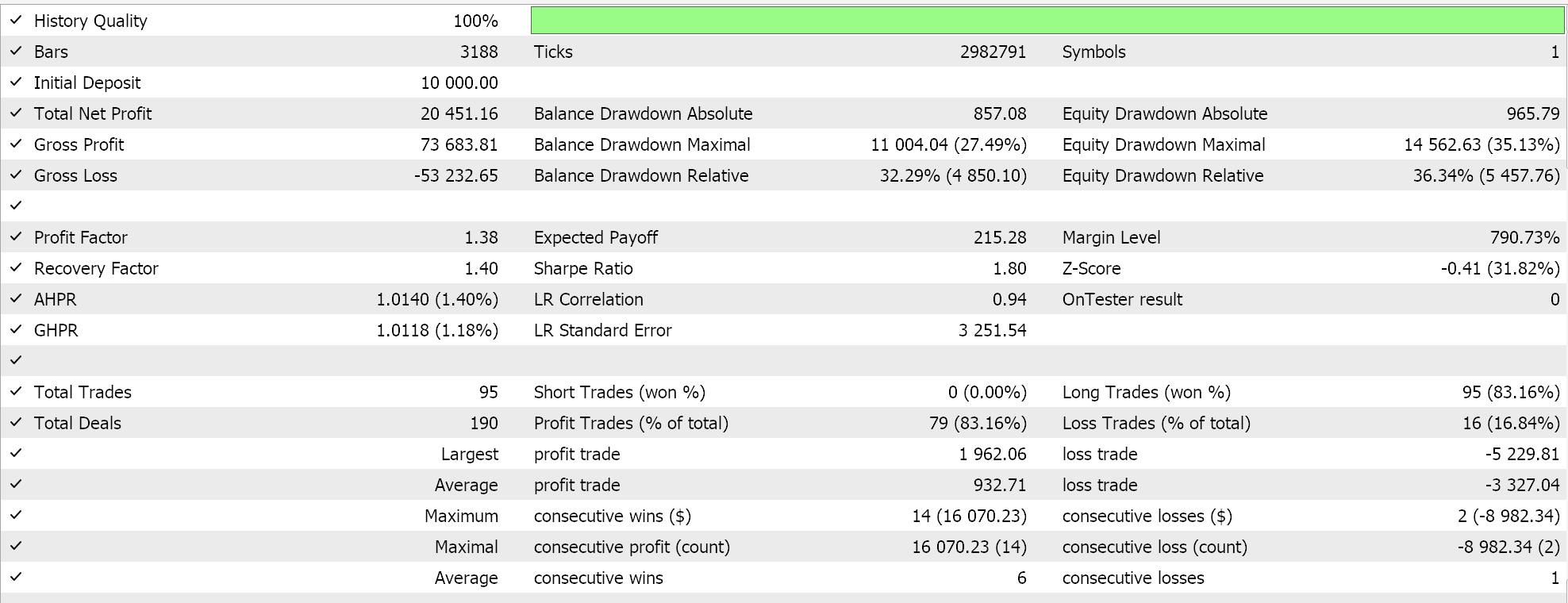
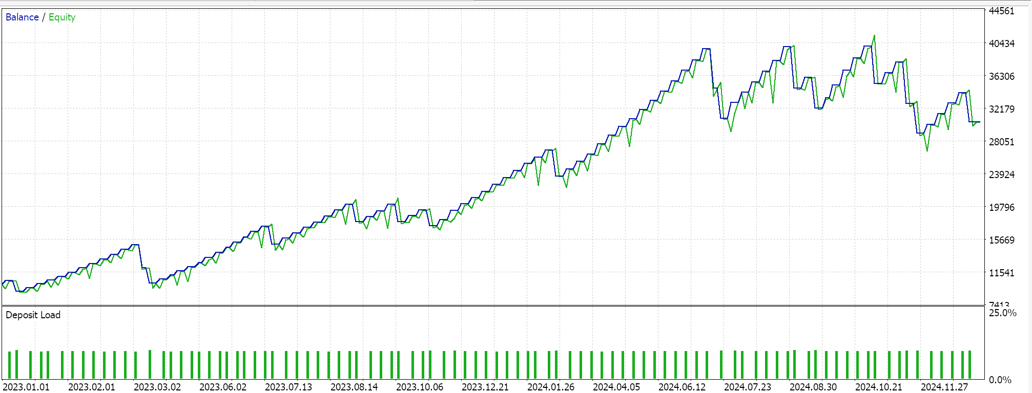
This anchor class, for all these functions, inherits from the ‘CExpertSignal’ base class for signal processing of MQL5 Expert Advisors. This allows integration with the ecosystem or class files used by wizard assembled Expert Advisors. We train, our 3 models for each of the patterns that were able to forward walk; 1, 4, and 5 and on importing to MQL5, test runs present us with the following reports:

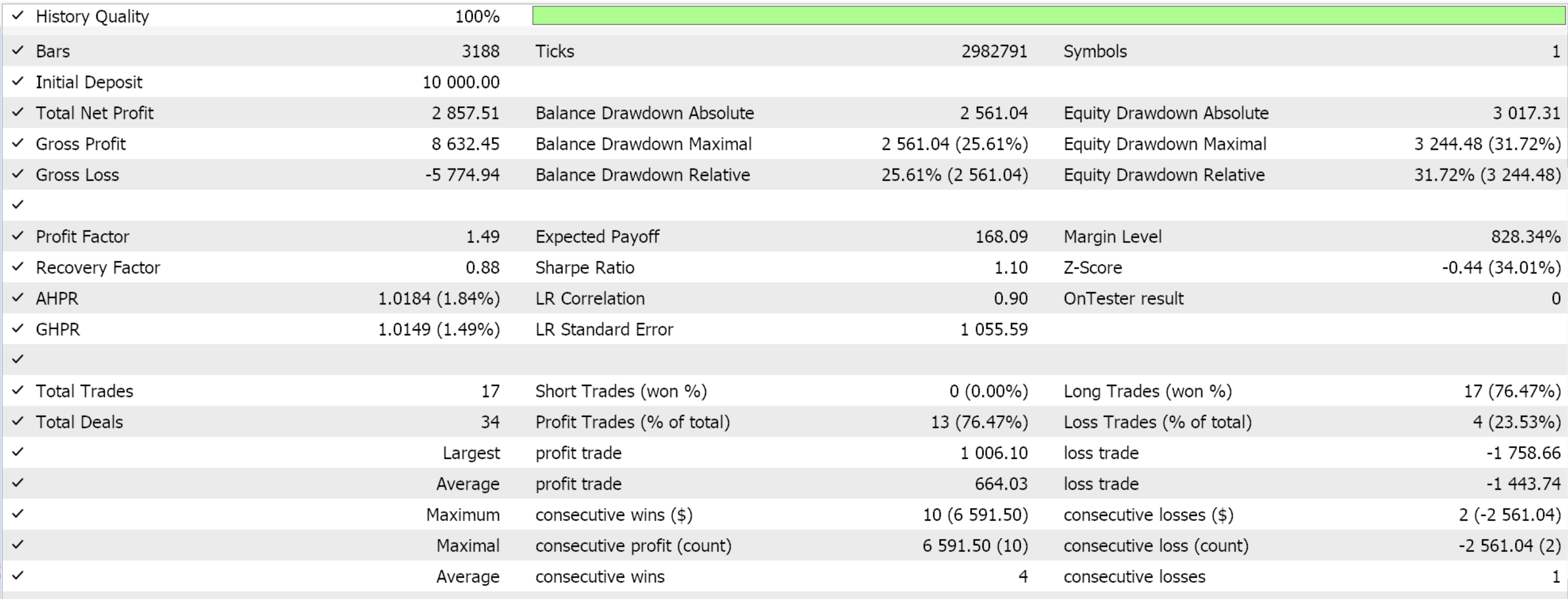
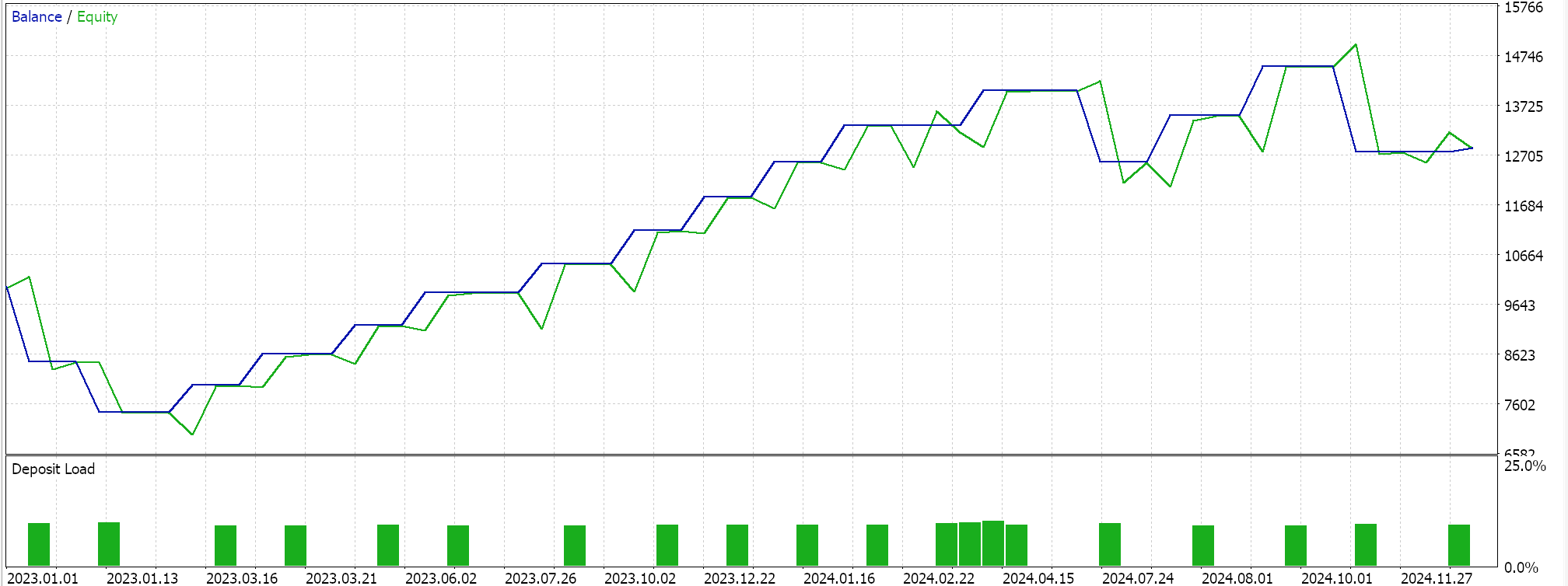
For Pattern-1

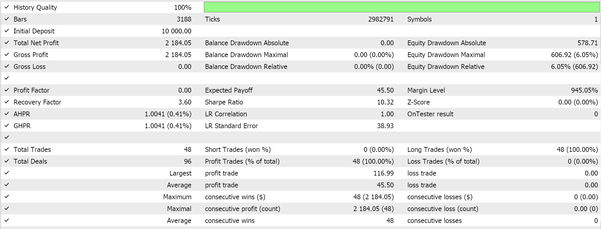
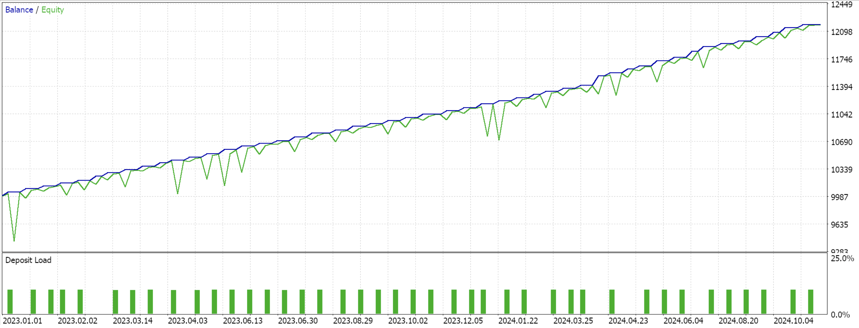
For Pattern-4

For Pattern-5

For new readers, there is an introductory guide here, with secondary links on how to use the attached code to assemble an Expert Advisor via the MQL5 wizard. The custom signal class we have created is designed for easy integration with the MQL5 wizard, and this makes it reusable across different Expert Advisors. ML integration is now a thing because we can use ONNX models to enhance Expert Advisor predictive capabilities. This does require, a robust set of training data. Validation of models with out-of-sample testing is important to avoid over fitting, and that's why for our exhibition purposes we use a 50/50 split on our data by training over one year and forward walking on the next.

From the test runs it appears all the patterns 1, 4, and 5 were able to walk, although only 4 it appears did so more ‘convincingly’. These test runs have major caveats, besides the short test window. Chief among them would be that testing is performed where open positions have a take profit price target without a stop-loss. The use of limit orders to make entries also makes these results a bit rosier than they would be otherwise. All these are considerations that the reader should bear in mind when interpreting or evaluating whether to further develop the source code that is attached.

Conclusion

We have looked at how the signals of the Triple Exponential Moving Average Oscillator can be combined with the Williams Percent Range Oscillator and processed by a machine learning model to make forecasts. Because the patterns we have considered had already walked, our machine learning model essentially acted as a filter over trades that we knew could forward walk for their test year. Performance improved, marginally, however in future articles we will consider testing with ML patterns that were unable to forward walk as well.

Name	Description
wz-68.mq5	Wizard assembled Expert Advisor whose header outlines files used in the assembly
SignalWZ_68.mqh	Custom signal class file used in the wizard assembly.
68_1.mqh	Exported ONNX model for pattern 1
68_4.mqh	Exported ONNX model for pattern 4
68_5.mqh	Exported ONNX model for pattern 5