Cross-validation and basics of causal inference in CatBoost models, export to ONNX format

Introduction

In the previous articles, I have described various ways to use machine learning algorithms to create trading systems. Some turned out to be quite successful, others (mostly from early publications) were greatly overtrained. Thus, the sequence of my articles reflects the evolution of understanding: what machine learning is actually capable of. We are, of course, talking about the classification of time series.

For example, the previous article "Metamodels in machine learning" considered the algorithm for finding patterns through the interaction of two classifiers. This non-trivial method was chosen due to the fact that ML algorithms are able to generalize and predict well, but are "lazy" in relation to the search for cause-and-effect relationships. In other words, they generalize training examples in which a cause-and-effect relationship may already be established that persists with new data, but this connection may also turn out to be associative, that is, passing and unreliable. 

The model does not understand what connections it is dealing with. It perceives all training data just as that - training data. This is a big problem for beginners trying to teach it how to trade profitably with new data. Therefore, in the last article an attempt was made to teach the algorithm to analyze its own errors in order to separate statistically significant predictions from random ones.

The current article is a development of the previous topic and the next step towards creating a self-training algorithm that is able to look for patterns in data while minimizing overfitting. After all, we want to get a real effect from the use of machine learning, so that it not only generalizes training examples, but also determines the presence of cause-and-effect relationships in them.

YIN (theory)

This section will contain a certain amount of subjective reasoning based on a bit of experience gained as a result of attempts to create "Artificial Intelligence" in Forex. Because it is not love yet, but it is still an experience. 

Just as our conclusions are often wrong and need to be verified, the results of predictions from machine learning models should be double-checked. If we turn the process of double-checking on ourselves, we get self-control. Self-control of machine learning model comes down to checking its predictions for errors many times in different but similar situations. If the model makes few errors on average, it means it is not overtrained, but if it makes mistakes often, then there is something wrong with it.

If we train the model once on selected data, then it cannot perform self-control. If we train a model many times on random subsamples, and then check the quality of the prediction on each and add up all the errors, we get a relatively reliable picture of the cases where it actually turns out to be wrong and the cases it often gets right. These cases can be divided into two groups and separated from each other. This is similar to conducting walk-forward validation or cross-validation, but with additional elements. This is the only way to achieve self-control and obtain a more robust model.

Therefore, it is necessary to conduct cross-validation on the training dataset, compare the model’s predictions with training labels and average the results across all folds. Those examples that were predicted incorrectly on average should be removed from the final training set as erroneous. We should also train a second model on all the data, which distinguishes well-predictable cases from poorly predictable ones, allowing us to cover all possible outcomes more fully. 

When bad training examples are removed, the main model will have a small classification error, but will perform poorly at predicting the cases that were removed. It will have high accuracy, but low recall. If we now add a second classifier and teach it to allow the first model to trade only in those cases that the first model has learned to classify well, then it should improve the results of the entire TS, since it has lower accuracy but higher recall.

It turns out that the errors of the first model are transferred to the second classifier, but do not disappear anywhere, so now it will make incorrect predictions more often. But due to the fact that it does not directly predict the direction of the transaction and the data coverage is greater, such predictions are still valuable.

We will assume that two models are sufficient to compensate for training errors with their positive results.

So, by eliminating bad training examples, we will look for situations that, on average, bring profit. And we will try not to trade in places that, on average, cause losses.

Algorithm core

The "meta learner" function is the core of the algorithm and does all of the above, so it should be analyzed in more detail. The remaining functions are auxiliary.

def meta_learner(folds_number: int, iter: int, depth: int, l_rate: float) -> pd.DataFrame:
    dataset = get_labels(get_prices())
    data = dataset[(dataset.index < FORWARD) & (dataset.index > BACKWARD)].copy()

    X = data[data.columns[1:-2]]
    y = data['labels']

    B_S_B = pd.DatetimeIndex([])

    # learn meta model with CV method
    meta_model = CatBoostClassifier(iterations = iter,
                                max_depth = depth,
                                learning_rate=l_rate,
                                verbose = False)
    
    predicted = cross_val_predict(meta_model, X, y, method='predict_proba', cv=folds_number)
    
    coreset = X.copy()
    coreset['labels'] = y
    coreset['labels_pred'] = [x[0] < 0.5 for x in predicted]
    coreset['labels_pred'] = coreset['labels_pred'].apply(lambda x: 0 if x < 0.5 else 1)
    
    # select bad samples (bad labels indices)
    diff_negatives = coreset['labels'] != coreset['labels_pred']
    B_S_B = B_S_B.append(diff_negatives[diff_negatives == True].index)
    to_mark = B_S_B.value_counts()
    marked_idx = to_mark.index
    data.loc[data.index.isin(marked_idx), 'meta_labels'] = 0.0
    return data[data.columns[1:]]

It accepts:

• number of folds for cross-validation
• number of training iterations for the base learner
• depth of the base learner tree
• gradient step

These parameters affect the final result and should be selected empirically or using a grid. 

The cross_val_predict function of the scikit learn package returns cross-validation scores for each training example, and then compares these scores to the original labels. If the predictions are incorrect, they are entered into the book of bad examples, on the basis of which "meta labels" are then generated for the second classifier.

The function returns the dataframe passed to it with additional "meta labels". This dataframe is then used to train the final models, as shown in the listing.

# features for model\meta models. We learn main model only on filtered labels 
    X, X_meta = dataset[dataset['meta_labels']==1], dataset[dataset.columns[:-2]]
    X = X[X.columns[:-2]]
    
    # labels for model\meta models
    y, y_meta = dataset[dataset['meta_labels']==1], dataset[dataset.columns[-1]]
    y = y[y.columns[-2]]

It is noted in the code above that the first model is trained only on those lines whose meta labels correspond to one, that is, they are marked as good training examples. The second classifier is trained on the entire dataset.

Then two classifiers are simply trained. One predicts the probabilities of buying and selling, while the second one determines whether it is worth trading or not.

Here, each model also has its own training parameters, which are not included in the hyperparameters. These can be configured separately, but I deliberately chose a small number of iterations equal to 100, so that the models do not overtrain at this final stage. We can change the relative sizes of the train and test samples, which will also slightly affect the final results. In general, the first model is quite easy to train, since it is trained only on examples that are well classified. Much complexity in the model is not required. The second model has a more complex task, so the complexity of the model can be increased.

# train\test split
    train_X, test_X, train_y, test_y = train_test_split(
        X, y, train_size=0.5, test_size=0.5, shuffle=True)
    
    train_X_m, test_X_m, train_y_m, test_y_m = train_test_split(
        X_meta, y_meta, train_size=0.5, test_size=0.5, shuffle=True)

    # learn main model with train and validation subsets
    model = CatBoostClassifier(iterations=100,
                               custom_loss=['Accuracy'],
                               eval_metric='Accuracy',
                               verbose=False,
                               use_best_model=True,
                               task_type='CPU')
    model.fit(train_X, train_y, eval_set=(test_X, test_y),
              early_stopping_rounds=15, plot=False)
    
    # learn meta model with train and validation subsets
    meta_model = CatBoostClassifier(iterations=100,
                                    custom_loss=['Accuracy'],
                                    eval_metric='Accuracy',
                                    verbose=False,
                                    use_best_model=True,
                                    task_type='CPU')
    meta_model.fit(train_X_m, train_y_m, eval_set=(test_X_m, test_y_m),
              early_stopping_rounds=15, plot=False)

Algorithm hyperparameters

Before starting training, we should correctly configure all input parameters, which also affect the final result.

export_path = '/Users/dmitrievsky/Library/Application Support/MetaTrader 5/\
Bottles/metatrader5/drive_c/Program Files/MetaTrader 5/MQL5/Include/'

# GLOBALS
SYMBOL = 'EURUSD'
MARKUP = 0.00015
PERIODS = [i for i in range(10, 50, 10)]
BACKWARD = datetime(2015, 1, 1)
FORWARD = datetime(2022, 1, 1)

• Path to the Include terminal folder for saving trained models
• Symbol ticker
• Average markup in points, including spread, commissions and slippages
• Moving average periods used to calculate price increments. These are attributes for training the model.
• Date range for training. To the left and right of this range is the history without training (OOS) for tests on new data.

def get_labels(dataset, min= 3, max= 25) -> pd.DataFrame:

This function has 'min' and 'max' arguments to randomly sample trades. Each new trade will have a random duration in bars. If we set the same values, then all trades will have a fixed duration. 

Auxiliary functions and libraries

Before we begin, make sure that all required packages are installed and imported

import numpy as np
import pandas as pd
import random
import math
from datetime import datetime
import matplotlib.pyplot as put
from catboost import CatBoostClassifier
from sklearn.model_selection import train_test_split
from sklearn.linear_model import LinearRegression
from sklearn.model_selection import cross_val_predict

Next, we should export quotes from the MetaTrader 5 terminal. Select the required symbol, timeframe and history depth and save them to the /files subdirectory of your Python project.

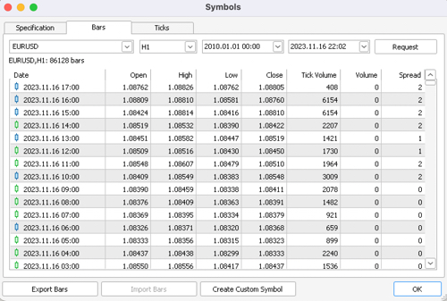
def get_prices() -> pd.DataFrame:
    p = pd.read_csv('files/EURUSD_H1.csv', delim_whitespace=True)
    pFixed = pd.DataFrame(columns=['time', 'close'])
    pFixed['time'] = p['<DATE>'] + ' ' + p['<TIME>']
    pFixed['time'] = pd.to_datetime(pFixed['time'], format='mixed')
    pFixed['close'] = p['<CLOSE>']
    pFixed.set_index('time', inplace=True)
    pFixed.index = pd.to_datetime(pFixed.index, unit='s')
    pFixed = pFixed.dropna()
    pFixedC = pFixed.copy()

    count = 0
    for i in PERIODS:
        pFixed[str(count)] = pFixedC.rolling(i).mean() - pFixedC
        count += 1

    return pFixed.dropna()

The highlighted code shows where the bot gets quotes from and how it creates attributes - by subtracting close prices from the moving average specified in the PERIODS list as a hyperparameter.

After that, the generated dataset is passed to the next function for marking labels (or targets).

def get_labels(dataset, min= 3, max= 25) -> pd.DataFrame:
    labels = []
    meta_labels = []
    for i in range(dataset.shape[0]-max):
        rand = random.randint(min, max)
        curr_pr = dataset['close'][i]
        future_pr = dataset['close'][i + rand]

        if future_pr < curr_pr:
            labels.append(1.0)
            if future_pr + MARKUP < curr_pr:
                meta_labels.append(1.0)
            else:
                meta_labels.append(0.0)
        elif future_pr > curr_pr:
            labels.append(0.0)
            if future_pr - MARKUP > curr_pr:
                meta_labels.append(1.0)
            else:
                meta_labels.append(0.0)
        else:
            labels.append(2.0)
            meta_labels.append(0.0)
        
    dataset = dataset.iloc[:len(labels)].copy()
    dataset['labels'] = labels
    dataset['meta_labels'] = meta_labels
    dataset = dataset.dropna()
    dataset = dataset.drop(
        dataset[dataset.labels == 2.0].index)
    
    return dataset

This function returns the same dataframe, but with additional "labels" and "meta labels" columns.

The tester function has been significantly accelerated. Now we can load large datasets and not worry that the tester will work too slowly:

def tester(dataset: pd.DataFrame, plot= False):
    last_deal = int(2)
    last_price = 0.0
    report = [0.0]
    chart = [0.0]
    line = 0
    line2 = 0

    indexes = pd.DatetimeIndex(dataset.index)
    labels = dataset['labels'].to_numpy()
    metalabels = dataset['meta_labels'].to_numpy()
    close = dataset['close'].to_numpy()

    for i in range(dataset.shape[0]):
        if indexes[i] <= FORWARD:
            line = len(report)
        if indexes[i] <= BACKWARD:
            line2 = len(report)

        pred = labels[i]
        pr = close[i]
        pred_meta = metalabels[i] # 1 = allow trades

        if last_deal == 2 and pred_meta==1:
            last_price = pr
            last_deal = 0 if pred <= 0.5 else 1
            continue

        if last_deal == 0 and pred > 0.5 and pred_meta == 1:
            last_deal = 2
            report.append(report[-1] - MARKUP + (pr - last_price))
            chart.append(chart[-1] + (pr - last_price))
            continue

        if last_deal == 1 and pred < 0.5 and pred_meta==1:
            last_deal = 2
            report.append(report[-1] - MARKUP + (last_price - pr))
            chart.append(chart[-1] + (pr - last_price))

    y = np.array(report).reshape(-1, 1)
    X = np.arange(len(report)).reshape(-1, 1)
    lr = LinearRegression()
    lr.fit(X, y)

    l = lr.coef_
    if l >= 0:
        l = 1
    else:
        l = -1

    if(plot):
        plt.plot(report)
        plt.plot(chart)
        plt.axvline(x = line, color='purple', ls=':', lw=1, label='OOS')
        plt.axvline(x = line2, color='red', ls=':', lw=1, label='OOS2')
        plt.plot(lr.predict(X))
        plt.title("Strategy performance R^2 " + str(format(lr.score(X, y) * l,".2f")))
        plt.xlabel("the number of trades")
        plt.ylabel("cumulative profit in pips")
        plt.show()

    return lr.score(X, y) * l

The auxiliary function for testing already trained models now has a more concise appearance. It takes a list of models as input, calculates class probabilities and passes them to the tester in the same way as if it were a ready-made dataframe with features and labels for testing. Therefore, the tester itself works both with the original training dataframes and with those generated as a result of receiving forecasts from already trained models.

def test_model(result: list, plt= False):
    pr_tst = get_prices()
    X = pr_tst[pr_tst.columns[1:]]
    pr_tst['labels'] = result[0].predict_proba(X)[:,1]
    pr_tst['meta_labels'] = result[1].predict_proba(X)[:,1]
    pr_tst['labels'] = pr_tst['labels'].apply(lambda x: 0.0 if x < 0.5 else 1.0)
    pr_tst['meta_labels'] = pr_tst['meta_labels'].apply(lambda x: 0.0 if x < 0.5 else 1.0)

    return tester(pr_tst, plot=plt)

YANG (practice)

After setting up the hyperparameters, we proceed directly to training the models, which is performed in a loop.

options = []
for i in range(25):
    print('Learn ' + str(i) + ' model')
    options.append(learn_final_models(meta_learner(folds_number= 5, iter= 150, depth= 5, l_rate= 0.01)))

options.sort(key=lambda x: x[0])
test_model(options[-1][1:], plt=True)

Here we will train 25 models, after which we will test them and export them to the MetaTrader 5 terminal.

The training results are most strongly influenced by the selected parameters, as well as the range of dates for training and testing, as well as the duration of transactions. We should experiment with these settings.

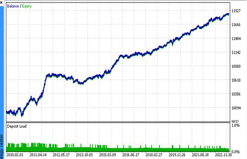
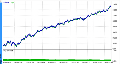
Let's look at the top 5 best models according to R^2 taking into account new data. The horizontal lines in the graphs show the OOS on the left and right.

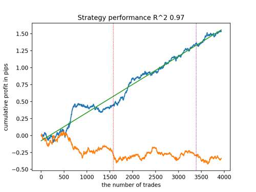
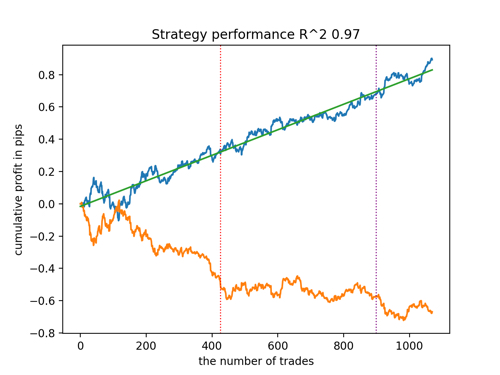
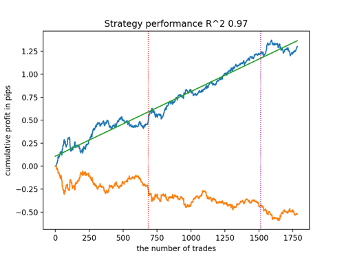
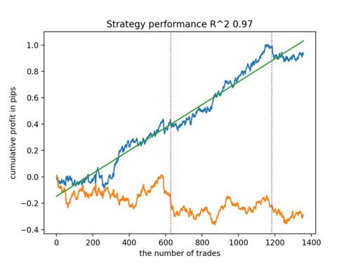
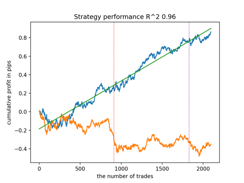
The balance graph is shown in blue, and the quotes graph is shown in orange. We can see that all models are different from each other. This is due to random sampling of transactions, as well as randomization built into each model. However, these models no longer look like testing grails and work quite confidently in OOS. In addition, we can compare the number of transactions, profit in points and the general appearance of the curves. Of course, the first and second models compare favorably, so we export them to the terminal.

It should be borne in mind that by changing the training parameters and doing several restarts, we will get unique behavior. The graphs will almost never be identical, but a significant part of them (which is important) will show well on the OOS.

Exporting the model to ONNX format

In previous articles, I used parsing models from cpp to MQL. Currently, the MetaTrader 5 terminal supports importing models into the ONNX format. This is quite convenient because you can write less code and transfer almost any model trained in Python.

The CatBoost algorithm has its own method of exporting models in ONNX format. Let's look at the export process in more detail.

At the output, we have two CatBoost models and a function that generates features in the form of increments. Since the function is quite simple, we will simply transfer it into the bot code, while the models will be exported to ONNX files.

def export_model_to_ONNX(model, model_number):
    model[1].save_model(
    export_path +'catmodel' + str(model_number) +'.onnx',
    format="onnx",
    export_parameters={
        'onnx_domain': 'ai.catboost',
        'onnx_model_version': 1,
        'onnx_doc_string': 'test model for BinaryClassification',
        'onnx_graph_name': 'CatBoostModel_for_BinaryClassification'
    },
    pool=None)

    model[2].save_model(
    export_path + 'catmodel_m' + str(model_number) +'.onnx',
    format="onnx",
    export_parameters={
        'onnx_domain': 'ai.catboost',
        'onnx_model_version': 1,
        'onnx_doc_string': 'test model for BinaryClassification',
        'onnx_graph_name': 'CatBoostModel_for_BinaryClassification'
    },
    pool=None)
    
    code = '#include <Math\Stat\Math.mqh>'
    code += '\n'
    code += '#resource "catmodel'+str(model_number)+'.onnx" as uchar ExtModel[]'
    code += '\n'
    code += '#resource "catmodel_m'+str(model_number)+'.onnx" as uchar ExtModel2[]'
    code += '\n'
    code += 'int Periods' + '[' + str(len(PERIODS)) + \
        '] = {' + ','.join(map(str, PERIODS)) + '};'
    code += '\n\n'

    # get features
    code += 'void fill_arays' + '( double &features[]) {\n'
    code += '   double pr[], ret[];\n'
    code += '   ArrayResize(ret, 1);\n'
    code += '   for(int i=ArraySize(Periods'')-1; i>=0; i--) {\n'
    code += '       CopyClose(NULL,PERIOD_H1,1,Periods''[i],pr);\n'
    code += '       ret[0] = MathMean(pr) - pr[Periods[i]-1];\n'
    code += '       ArrayInsert(features, ret, ArraySize(features), 0, WHOLE_ARRAY); }\n'
    code += '   ArraySetAsSeries(features, true);\n'
    code += '}\n\n'

    file = open(export_path + str(SYMBOL) + ' ONNX include' + str(model_number) + '.mqh', "w")
    file.write(code)

    file.close()
    print('The file ' + 'ONNX include' + '.mqh ' + 'has been written to disk')

The export function receives a list of models. Each of them is stored in ONNX with optional export parameters. All this code saves the models into the Include folder of the terminal and also generates a .mqh file that looks something like this:

#resource "catmodel.onnx" as uchar ExtModel[]
#resource "catmodel_m.onnx" as uchar ExtModel2[]

#include <Math\Stat\Math.mqh>
int Periods[4] = {10,20,30,40};

void fill_arays( double &features[]) {
   double pr[], ret[];
   ArrayResize(ret, 1);
   for(int i=ArraySize(Periods)-1; i>=0; i--) {
       CopyClose(NULL,PERIOD_H1,1,Periods[i],pr);
       ret[0] = MathMean(pr) - pr[Periods[i]-1];
       ArrayInsert(features, ret, ArraySize(features), 0, WHOLE_ARRAY); }
   ArraySetAsSeries(features, true);
}

Next, we need to connect it to the bot. Each file has a unique name specified through the symbol ticker and the model serial number at the end. Therefore, we can store a collection of such trained models on disk, or connect several models to the bot at once. I will limit myself to one file for demonstration purposes.

#include <EURUSD ONNX include1.mqh>

In the function, we need to initialize the models correctly as shown below.  The most important thing is to correctly set the dimensions of the input and output data. Our models have a feature vector of variable length depending on the number of features that are specified in the PERIODS list or exported array, so we define the dimension of the input vector as shown below. Both models take the same number of features as input.

The dimension of the output vector may cause some confusion. 

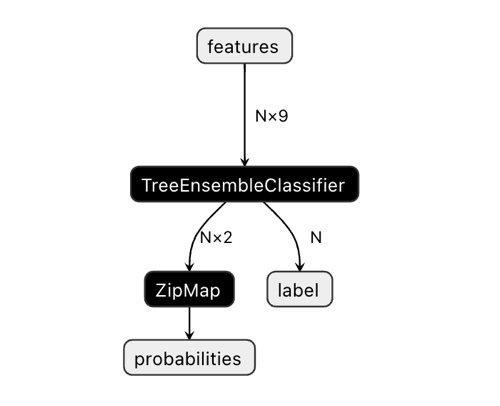
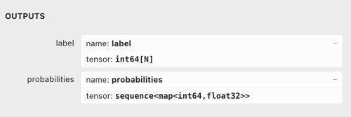
In the Netron application, we can see that the model has two outputs. The first one is a unit tensor with class labels defined later in the code as a zero output or zero index output. But it cannot be used to make predictions because there are known issues described in the CatBoost documentation:

"The label is inferred incorrectly for binary classification. This is a known bug in the onnxruntime implementation. Ignore the value of this parameter in case of binary classification."

Accordingly, we should use the second "probabilities" output, but I was unable to set it correctly in the MQL code, so I simply did not define it. However, it was defined on its own and everything works. I have no idea why.

Therefore, the second output is used to obtain class probabilities in the bot.

const long  ExtInputShape [] = {1, ArraySize(Periods)};

int OnInit() {
   ExtHandle = OnnxCreateFromBuffer(ExtModel, ONNX_DEFAULT);
   ExtHandle2 = OnnxCreateFromBuffer(ExtModel2, ONNX_DEFAULT);

   if(ExtHandle == INVALID_HANDLE || ExtHandle2 == INVALID_HANDLE) {
      Print("OnnxCreateFromBuffer error ", GetLastError());
      return(INIT_FAILED);
   }

   if(!OnnxSetInputShape(ExtHandle, 0, ExtInputShape)) {
      Print("OnnxSetInputShape failed, error ", GetLastError());
      OnnxRelease(ExtHandle);
      return(-1);
   }

   if(!OnnxSetInputShape(ExtHandle2, 0, ExtInputShape)) {
      Print("OnnxSetInputShape failed, error ", GetLastError());
      OnnxRelease(ExtHandle2);
      return(-1);
   }

   const long output_shape[] = {1};
   if(!OnnxSetOutputShape(ExtHandle, 0, output_shape)) {
      Print("OnnxSetOutputShape error ", GetLastError());
      return(INIT_FAILED);
   }
   if(!OnnxSetOutputShape(ExtHandle2, 0, output_shape)) {
      Print("OnnxSetOutputShape error ", GetLastError());
      return(INIT_FAILED);
   }

   return(INIT_SUCCEEDED);
}

Receiving model signals is implemented in this way. Here we declare an array of features and fill it through the fill_arrays() function located in the exported .mqh file.

Next, I declared another array f to invert the order of the features array values, and submitted it to Onnx Runtime for execution. The first output as a vector just needs to be passed in, but we will not use it. The array of structures is passed as the second output.

The models (main and meta) are executed and return predicted values to the tensor array. I take second-class probabilities from it.

void OnTick() {
   if(!isNewBar())
      return;

   double features[];
   fill_arays(features);

   double f[ArraySize(Periods)];

   int k = ArraySize(Periods) - 1;
   for(int i = 0; i < ArraySize(Periods); i++) {
      f[i] = features[i];
      k--;
   }

   static vector out(1), out_meta(1);

   struct output {
      long           label[];
      float          tensor[];
   };

   output out2[], out2_meta[];

   OnnxRun(ExtHandle, ONNX_DEBUG_LOGS, f, out, out2);
   OnnxRun(ExtHandle2, ONNX_DEBUG_LOGS, f, out_meta, out2_meta);

   double sig = out2[0].tensor[1];
   double meta_sig = out2_meta[0].tensor[1];

The rest of the bot code should be familiar to you from the previous article. We check the meta_sig enabling signal. If it is greater than 0.5, then opening and closing deals is allowed depending on the direction specified by the sig signal of the first model.

if(meta_sig > 0.5)
      if(count_market_orders(0) || count_market_orders(1))
         for(int b = OrdersTotal() - 1; b >= 0; b--)
            if(OrderSelect(b, SELECT_BY_POS) == true) {
               if(OrderType() == 0 && OrderSymbol() == _Symbol && OrderMagicNumber() == OrderMagic && sig > 0.5)
                  if(SymbolInfoInteger(_Symbol, SYMBOL_TRADE_FREEZE_LEVEL) < MathAbs(Bid - OrderOpenPrice())) {
                     int res = -1;
                     do {
                        res = OrderClose(OrderTicket(), OrderLots(), OrderClosePrice(), 0, Red);
                        Sleep(50);
                     } while (res == -1);
                  }
               if(OrderType() == 1 && OrderSymbol() == _Symbol && OrderMagicNumber() == OrderMagic && sig < 0.5)
                  if(SymbolInfoInteger(_Symbol, SYMBOL_TRADE_FREEZE_LEVEL) < MathAbs(Bid - OrderOpenPrice())) {
                     int res = -1;
                     do {
                        res = OrderClose(OrderTicket(), OrderLots(), OrderClosePrice(), 0, Red);
                        Sleep(50);
                     } while (res == -1);
                  }
            }


   if(meta_sig > 0.5)
      if(countOrders() < max_orders && CheckMoneyForTrade(_Symbol, LotsOptimized(meta_sig), ORDER_TYPE_BUY)) {
         double l = LotsOptimized(meta_sig);
         if(sig < 0.5) {
            int res = -1;
            do {
               double stop = Bid - stoploss * _Point;
               double take = Ask + takeprofit * _Point;
               res = OrderSend(Symbol(), OP_BUY, l, Ask, 0, stop, take, comment, OrderMagic);
               Sleep(50);
            } while (res == -1);
         } else {
            if(sig > 0.5) {
               int res = -1;
               do {
                  double stop = Ask + stoploss * _Point;
                  double take = Bid - takeprofit * _Point;
                  res = OrderSend(Symbol(), OP_SELL, l, Bid, 0, stop, take, comment, OrderMagic);
                  Sleep(50);
               } while (res == -1);
            }
         }
      }

Final tests

Let's sequentially connect 2 files with the models we like and make sure that the results of the custom tester completely coincide with the results of the MetaTrader 5 tester.

Additionally, we can test the bots on real ticks, optimize stop loss and take profit, select the lot size and add more deals in the MetaTrader 5 optimizer.

Final word

I don’t know if there is a scientific basis for this approach to classifying time series for trading tasks. It was invented by trial and error and seemed quite interesting and promising to me.

With this little study, I wanted to highlight that sometimes machine learning models should be trained in a different way than what seems obvious. In addition to a specific architecture, the way these models are applied is of great importance as well. At the same time, a statistical approach to analyzing training outcomes is coming to the fore, be it the fully automatic "trader and researcher" approach presented in this article, or simpler algorithms that require the expert intervention of a "Teacher".