
Neural networks made easy (Part 57): Stochastic Marginal Actor-Critic (SMAC)

Introduction
When building an automated trading system, we develop algorithms for sequential decision making. Reinforcement learning methods are aimed exactly at solving such problems. One of the key issues in reinforcement learning is the exploration process as the Agent learns to interact with its environment. In this context, the principle of maximum entropy is often used, which motivates the Agent to perform actions with the greatest degree of randomness. However, in practice, such algorithms train simple Agents that learn only local changes around a single action. This is due to the need to calculate the entropy of the Agent's policy and use it as part of the training goal.
At the same time, a relatively simple approach to increasing the expressiveness of an Actor's policy is to use latent variables, which provide the Agent with its own inference procedure to model stochasticity in observations, the environment and unknown rewards.
Introducing latent variables into the Agent's policy allows it to cover more diverse scenarios that are compatible with historical observations. It should be noted here that policies with latent variables do not allow a simple expression to determine their entropy. Naive entropy estimation can lead to catastrophic failures in policy optimization. Besides, high variance stochastic updates for entropy maximization do not readily distinguish between local random effects and multimodal exploration.
One of the options for solving these latent variable policies shortcomings was proposed in the article "Latent State Marginalization as a Low-cost Approach for Improving Exploration". The authors propose a simple yet effective policy optimization algorithm capable of providing more efficient and robust exploration in both fully observable and partially observable environments.
The main contributions of this article can be briefly summarized by the following theses:
- Motivation for using latent variable policies to improve exploration and robustness under conditions of partial observability.
- Several stochastic estimation methods are proposed that focus on study efficiency and variance reduction.
- Applying approaches to the Actor-Critic method leads to the creation of the Stochastic Marginal Actor-Critic (SMAC) algorithm.
1. SMAC algorithm
The authors of the Stochastic Marginal Actor-Critic algorithm algorithm propose to use latent variables to build a distributed Actor policy. This is a simple and efficient way to increase the flexibility of the Agent's action models and policies. This approach requires minimal changes to be implemented into existing algorithms using stochastic Agent behavior policies.
A latent variable policy can be expressed as follows:
![]()
where st is a latent variable that depends on the current observation.
Introduction of the q(st|xt) latent variable usually increases the expressiveness of the Actor's policies. This allows the policy to capture a wider range of optimal actions. This can be especially useful in the early stages of research when information about future rewards is lacking.
To parameterize the stochastic model, the authors of the method propose to use factorized Gaussian distributions both for the π(at|st) Actor policy, and for the q(st|xt) latent variable function. This results in a computationally efficient latent variable policy since sampling and density estimation remain inexpensive. In addition, it allows us to apply the proposed approaches to build models based on existing algorithms with stochastic policies and a single Gaussian distribution. We simply add a new st stochastic node.
Please note that due to Markov's assumption process, π(at|st) depends only on the current latent state, although the proposed algorithm can easily be extended to non-Markov situations. However, thanks to recurrence, we observe marginalization according to the complete hidden history since the current latent state st state, as well as the π(at|st) policy, are a consequence of a series of transitions from the initial state under the influence of actions performed by the Agent.
![]()
At the same time, the proposed approaches to processing latent variables do not depend on what q affects.
The presence of latent variables makes maximum entropy training quite difficult. After all, this requires an accurate assessment of the entropy component. The entropy of a latent variable model is extremely difficult to estimate due to the difficulty of marginalization. In addition, the use of latent variables increases the variance of the gradient. Also, latent variables can be used in the Q-function for better aggregation of uncertainty.
In each of these cases, the authors of Stochastic Marginal Actor-Critic derive reasonable methods for handling latent variables. The end result is quite simple and adds a minimal amount of additional resource costs compared to policies without latent variables.
In turn, the use of latent variables makes entropy (or marginal entropy) unusable due to the unsolvability of the probability logarithm.
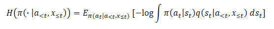
Using a naive estimator will result in maximizing the upper bound on the objective maximum entropy functional causing error maximization. This encourages the variation distribution to be as far as possible from the q(st|a<t,x≤t) true posterior estimate. Moreover, this error is not bounded and can become arbitrarily large without actually affecting the true entropy we want to maximize, leading to serious problems with numerical instability.
The article showcases the results of a preliminary experiment, in which this approach to estimating entropy during policy optimization resulted in extremely large values significantly overestimating the true entropy and leading to untrained policies. Below is a visualization from the mentioned article.
To overcome the overestimation issue, the method authors propose to construct an estimator of the lower bound of marginal entropy.

where p(st|a≤t,x≤t) is the unknown posterior distribution of the policy.
However, we can easily choose st⁰ from it and then select at if st⁰. This results in a nested evaluator where we actually select K+1 times out of q(st|a<t,x≤t). To select the action, we use only the first st⁰ latent variable. All other latent variables are used to estimate marginal entropy.
Note that this is not equivalent to replacing the expectation within the logarithm with independent samples. The proposed estimator increases monotonically with K, which in the limit becomes an unbiased marginal entropy estimator.
The above methods can be applied to general entropy maximization algorithms. But the method authors create a specific algorithm called Stochastic Marginal Actor-Critic (SMAC). SMAC is characterized by using an Actor policy with latent variables and maximizing the lower bound of the marginal entropy objective function.
The algorithm follows the generally accepted Actor-Critic style and uses the experience playback buffer to store data, based on which the parameters of both the Actor and the Critic are updated.
The critic learns by minimizing the error:
![]()
where:
(x, a, r, x') — from the D playback buffer,
a' — Actor's action according to the π(·|x') policy,
Q ̅ — Critic's target function,
H ̃ — policy entropy estimation.
In addition, we estimate policy entropy with latent variables.
Additionally, the Actor is updated by minimizing the error:
![]()
Note that when updating the critic, we use the entropy estimate of the Actor's policy in the subsequent state, while when updating the Actor's policy — in the current one.
Overall, SMAC is essentially the same as naive SAC in terms of the algorithmic details of reinforcement learning methods, but gains improvements primarily through structured exploration behavior. This is achieved through latent variable modeling.
2. Implementation using MQL5
Above are the theoretical calculations of the author's Stochastic Marginal Actor-Critic method. In the practical part of this article, we will implement the proposed algorithm using MQL5. The only exception is that we will not completely repeat the original SMAC algorithm. The mentioned article considers the possibility of using the proposed methods in almost all reinforcement learning algorithms. We will take advantage of this opportunity and implement the proposed methods in our implementation of the NNM algorithm we discussed in the previous article.
The first changes will be made to the architecture of the models. As we can see in the equations presented above, the SMAC algorithm is based on three models:
- q — model for representing the latent state;
- π — Actor;
- Q — Critic.
I think, the last two models do not raise any questions. The first latent state model is an Encoder with a stochastic node at the output. Both the Actor and the Critic use the Encoder operation results as source data. Here it would be appropriate to recall the variational auto Encoder.
Our existing developments allow us not to move the Encoder into a separate model, but to leave it, as before, within the architecture of the Actor model. Thus, to implement the proposed algorithm, we have to make changes to the Actor architecture. Namely, we need to add a stochastic node at the output of the data preprocessing block (Encoder).
The architecture of the models is specified in the CreateDescriptions method. Essentially, we are making minimal changes to the Actor architecture, while leaving the data preprocessing block unchanged. Historical data of price movement and indicators is fed to a fully connected neural layer. Then they undergo primary processing in the neural layer of batch normalization.
bool CreateDescriptions(CArrayObj *actor, CArrayObj *critic, CArrayObj *convolution)
  {
//---
   CLayerDescription *descr;
//---
   if(!actor)
     {
      actor = new CArrayObj();
      if(!actor)
         return false;
     }
   if(!critic)
     {
      critic = new CArrayObj();
      if(!critic)
         return false;
     }
   if(!convolution)
     {
      convolution = new CArrayObj();
      if(!convolution)
         return false;
     }
//--- Actor
   actor.Clear();
//--- Input layer
   if(!(descr = new CLayerDescription()))
      return false;
   descr.type = defNeuronBaseOCL;
   int prev_count = descr.count = (HistoryBars * BarDescr);
   descr.activation = None;
   descr.optimization = ADAM;
   if(!actor.Add(descr))
     {
      delete descr;
      return false;
     }
//--- layer 1
   if(!(descr = new CLayerDescription()))
      return false;
   descr.type = defNeuronBatchNormOCL;
   descr.count = prev_count;
   descr.batch = 1000;
   descr.activation = None;
   descr.optimization = ADAM;
   if(!actor.Add(descr))
     {
      delete descr;
      return false;
     }
The normalized data is then passed through two successive convolutional layers, in which we try to extract certain patterns from the data structure.
//--- layer 2
   if(!(descr = new CLayerDescription()))
      return false;
   descr.type = defNeuronConvOCL;
   prev_count = descr.count = BarDescr;
   descr.window = HistoryBars;
   descr.step = HistoryBars;
   int prev_wout = descr.window_out = HistoryBars / 2;
   descr.activation = LReLU;
   descr.optimization = ADAM;
   if(!actor.Add(descr))
     {
      delete descr;
      return false;
     }
//--- layer 3
   if(!(descr = new CLayerDescription()))
      return false;
   descr.type = defNeuronConvOCL;
   prev_count = descr.count = prev_count;
   descr.window = prev_wout;
   descr.step = prev_wout;
   descr.window_out = 8;
   descr.activation = LReLU;
   descr.optimization = ADAM;
   if(!actor.Add(descr))
     {
      delete descr;
      return false;
     }
We marginalize the state of the environment with two fully connected layers.
//--- layer 4
   if(!(descr = new CLayerDescription()))
      return false;
   descr.type = defNeuronBaseOCL;
   descr.count = LatentCount;
   descr.optimization = ADAM;
   descr.activation = LReLU;
   if(!actor.Add(descr))
     {
      delete descr;
      return false;
     }
//--- layer 5
   if(!(descr = new CLayerDescription()))
      return false;
   descr.type = defNeuronBaseOCL;
   prev_count = descr.count = LatentCount;
   descr.activation = LReLU;
   descr.optimization = ADAM;
   if(!actor.Add(descr))
     {
      delete descr;
      return false;
     }
Next, we combine the received data with information about the account status. Here we make the first change to the model architecture. Before the stochastic block, we need to create a layer twice the size of the latent representation: we need measures of the distribution in the form of means and variances. Therefore, we specify the size of the concatenation layer to be twice the size of the latent representation. It is followed by the layer of the latent state of the variational auto encoder. It is with this layer that we create a stochastic node.
//--- layer 6
   if(!(descr = new CLayerDescription()))
      return false;
   descr.type = defNeuronConcatenate;
   descr.count = 2 * LatentCount;
   descr.window = prev_count;
   descr.step = AccountDescr;
   descr.optimization = ADAM;
   descr.activation = SIGMOID;
   if(!actor.Add(descr))
     {
      delete descr;
      return false;
     }
//--- layer 7
   if(!(descr = new CLayerDescription()))
      return false;
   descr.type = defNeuronVAEOCL;
   descr.count = LatentCount;
   descr.optimization = ADAM;
   if(!actor.Add(descr))
     {
      delete descr;
      return false;
     }
Please note that we have increased the size of our data preprocessing unit (Encoder). We have to take this into account when arranging data transfer between models.
I have left the Actor's decision-making block unchanged. It contains three fully connected layers and a latent state layer of a variational auto encoder, which creates stochastic behavior of the Actor.
//--- layer 8
   if(!(descr = new CLayerDescription()))
      return false;
   descr.type = defNeuronBaseOCL;
   descr.count = LatentCount;
   descr.activation = LReLU;
   descr.optimization = ADAM;
   if(!actor.Add(descr))
     {
      delete descr;
      return false;
     }
//--- layer 9
   if(!(descr = new CLayerDescription()))
      return false;
   descr.type = defNeuronBaseOCL;
   descr.count = LatentCount;
   descr.activation = LReLU;
   descr.optimization = ADAM;
   if(!actor.Add(descr))
     {
      delete descr;
      return false;
     }
//--- layer 10
   if(!(descr = new CLayerDescription()))
      return false;
   descr.type = defNeuronBaseOCL;
   descr.count = 2 * NActions;
   descr.activation = SIGMOID;
   descr.optimization = ADAM;
   if(!actor.Add(descr))
     {
      delete descr;
      return false;
     }
//--- layer 11
   if(!(descr = new CLayerDescription()))
      return false;
   descr.type = defNeuronVAEOCL;
   descr.count = NActions;
   descr.optimization = ADAM;
   if(!actor.Add(descr))
     {
      delete descr;
      return false;
     }
Now let's have a look at the Critic's architecture. At first glance, the proposals of the SMAC method authors do not contain requirements for the Critic’s architecture. We could easily leave it unchanged. As you might remember, we use a decomposed reward function. The question arises: where should we assign the entropy of the added stochastic node? We could add it to any of the existing reward elements. But in the context of decomposition of the reward function, it is more logical to add one more element at the output of the Critic. Therefore, we increase the constant of the number of reward elements.
#define NRewards 5 //Number of rewards
Other than that, the architecture of the Critic's model has remained unchanged.
//--- Critic
   critic.Clear();
//--- Input layer
   if(!(descr = new CLayerDescription()))
      return false;
   descr.type = defNeuronBaseOCL;
   prev_count = descr.count = LatentCount;
   descr.activation = None;
   descr.optimization = ADAM;
   if(!critic.Add(descr))
     {
      delete descr;
      return false;
     }
//--- layer 1
   if(!(descr = new CLayerDescription()))
      return false;
   descr.type = defNeuronConcatenate;
   descr.count = LatentCount;
   descr.window = prev_count;
   descr.step = NActions;
   descr.optimization = ADAM;
   descr.activation = LReLU;
   if(!critic.Add(descr))
     {
      delete descr;
      return false;
     }
//--- layer 2
   if(!(descr = new CLayerDescription()))
      return false;
   descr.type = defNeuronBaseOCL;
   descr.count = LatentCount;
   descr.activation = LReLU;
   descr.optimization = ADAM;
   if(!critic.Add(descr))
     {
      delete descr;
      return false;
     }
//--- layer 3
   if(!(descr = new CLayerDescription()))
      return false;
   descr.type = defNeuronBaseOCL;
   descr.count = LatentCount;
   descr.activation = LReLU;
   descr.optimization = ADAM;
   if(!critic.Add(descr))
     {
      delete descr;
      return false;
     }
//--- layer 4
   if(!(descr = new CLayerDescription()))
      return false;
   descr.type = defNeuronBaseOCL;
   descr.count = NRewards;
   descr.optimization = ADAM;
   descr.activation = None;
   if(!critic.Add(descr))
     {
      delete descr;
      return false;
     }
We have specified all the necessary models to implement the SMAC algorithm. However, do not forget that we are implementing the proposed methods into the NNM algorithm. Therefore, we keep all previously used models in order to preserve the full functionality of the algorithm. The Random Convolutional Encoder model is carried over without changes. I will not dwell on it. You can find it in the attachment. All programs used in this article are also presented there.
Let's return to the issue of data transfer between models. To let the Critic refer to the latent state of the Actor, we use the ID of the latent state layer specified in the LatentLayer constant. Therefore, in order to redirect the Critic to the desired neural layer in accordance with the change in the Actor’s architecture, we only need to change the value of the specified constant. No other adjustments to the program code are required in this context.
#define LatentLayer 7
Now let's discuss the use of algorithms for calculating the entropy component in the reward function. The method authors offered their vision of the issue presented in the theoretical part. However, we extend our implementation of the NNM method, in which we used the nuclear norm as the entropy component of the Actor. To make the values of various elements of the reward function comparable, it is logical to use a similar approach for the Encoder.
The authors of the SMAC method suggest using the K+1 Encoder sample to estimate the entropy of the latent state. It is obvious that for a single state of the environment during the Encoder training process we will arrive at some average value quite quickly. In the course of further optimization of the Encoder parameters, we will strive to reduce the variance value to maximize the separation of individual states. As the dispersion decreases in the limit to "0", the entropy will also tend to "0". Will we get the same effect using the kernel norm?
To answer this question, we may delve into math equations or we may refer to practice. Of course, we will not create and train a model for a long time now to test the possibility of using the kernel norm. We will make it much easier and faster. Let's create a small Python script.
First, let's import two libraries: numpy and matplotlib. We will use the first for calculations, and the second one - for visualizing the results.
# Import libraries
import numpy as np
import matplotlib.pyplot as plt
To create samples, we need statistical indicators of distributions: average values and corresponding variances. They will be generated by the model during training. We only need random values to test the approach.
mean = np.random.normal(size=[1,10])
std = np.random.rand(1,10)
Please note that any numbers can be used as averages. We generate them from a normal distribution. However, the variances can only be positive, and we generate them in the range (0, 1].
We will use the distribution re-parameterization trick similar to the stochastic node. To do this, we will generate a matrix of random values from the normal distribution.
data = np.random.normal(size=[20,10])
We will prepare a vector for recording our internal rewards.
reward=np.zeros([20])
The idea is as follows: we need to test how intrinsic rewards behave using the nuclear norm under reduced variance and other things being equal.
To reduce variance, we will create a vector of reduction factors.
scl = [2**(-k/2.0) for k in range(20)]
Next, we create a loop, in which we will use the distribution re-parameterization trick on our random data with constant means and decreasing variance. Based on the data obtained, we will calculate the internal reward using the kernel norm. Save the results obtained into the prepared reward vector.
for idx, k in enumerate(scl):
    new_data=mean+data*(std*k)
    _,S,_=np.linalg.svd(new_data)
    reward[idx]=S.sum()/(np.sqrt(new_data*new_data).sum()*max(new_data.shape))
Visualize the script results.
# Draw results
plt.plot(scl,reward)
plt.gca().invert_xaxis()
plt.ylabel('Reward')
plt.xlabel('STD multiplier')
plt.xscale('log',base=2)
plt.savefig("graph.png")
plt.show() 
The results obtained clearly demonstrate a decrease in internal reward using the kernel norm with a decrease in the distribution variance, all other things being equal. This means that we can safely use the kernel norm to estimate the entropy of the latent state.
Let's get back to our implementation of the algorithm using MQL5. Now we can start implementing the latent state entropy estimate. First, we need to determine the number of latent states to sample. We will define this indicator by the SamplLatentStates constant.
#define SamplLatentStates 32
The next question is: do we really need to do a full forward pass through the Encoder (in our case Actor) model to sample each latent state?
It is quite obvious that without changing the initial data and model parameters, the results of all neural layers will be identical with each subsequent pass. The only difference lies in the results of the stochastic node. Therefore, one direct pass of the Actor model is sufficient for us for each individual state. Next, we will use the distribution re-parameterization trick and sample the number of hidden states we need. I think, the idea is clear and we are moving on to implementation.
First, we generate a matrix of random values from a normal distribution with mean "0" and variance "1". Such distribution indicators are most convenient for re-parameterization.
float EntropyLatentState(CNet &net)
  {
//--- random values
   double random[];
   Math::MathRandomNormal(0,1,LatentCount * SamplLatentStates,random);
   matrix<float> states;
   states.Assign(random);
   states.Reshape(SamplLatentStates,LatentCount);
We will then load the trained distribution parameters from our Actor model, which are stored in the penultimate Encoder layer. It should be noted here that our model provides one data buffer, in which all the mean values of the learned distribution are sequentially stored, followed by all the variances. However, to perform matrix operations, we need two matrices with duplication of values along the rows, rather than one vector. Here we will use a little trick. First, we create one large matrix with the required number of rows and double the number of columns, filled with zero values. In the first line, we will write data from the data buffer with distribution parameters. Then we will use the function of cumulative summation of matrix values by columns.
The trick is that all strings except the first are filled with zeros. As a result of performing the cumulative sum operation, we will simply copy the data from the first row to all subsequent ones.
Now we simply divide the matrix into two equal ones vertically and get the array of split matrices. It will contain the matrix of average values with index 0. The variance matrix has the index of 1.
//--- get means and std
   vector<float> temp;
   matrix<float> stats = matrix<float>::Zeros(SamplLatentStates,2 * LatentCount);
   net.GetLayerOutput(LatentLayer - 1,temp);
   stats.Row(temp,0);
   stats=stats.CumSum(0);
   matrix<float> split[];
   stats.Vsplit(2,split);
Now we can quite simply re-parameterize random values from a normal distribution and get the number of samples we need.
//--- calculate latent values
   states = states * split[1] + split[0];
At the bottom of the matrix, we will add a string with the current Encoder values used by the Actor and Critics as input data during the forward pass.
//--- add current latent value
   net.GetLayerOutput(LatentLayer,temp);
   states.Resize(SamplLatentStates + 1,LatentCount);
   states.Row(temp,SamplLatentStates);
At this stage, we have all the data ready to calculate the kernel norm. We calculate the entropy component of the reward function. The result is returned to the calling program.
//--- calculate entropy
   states.SVD(split[0],split[1],temp);
   float result = temp.Sum() / (MathSqrt(MathPow(states,2.0f).Sum() *
                                MathMax(SamplLatentStates + 1,LatentCount)));
//---
   return result;
  }
The preparatory work is complete. Let's move on to working on EAs for interaction with the environment and training models.
The EAs for interaction with the environment (Research.mq5 and Test.mq5) have remained unchanged and we will not dwell on them now. The full code of all programs used in the article is available in the attachment.
Let's move on to the model training EA and focus on the Train training method. At the beginning of the method, we will determine the overall size of the experience playback buffer.
//+------------------------------------------------------------------+
//| Train function                                                   |
//+------------------------------------------------------------------+
void Train(void)
  {
   int total_tr = ArraySize(Buffer);
   uint ticks = GetTickCount();
Then we will encode all existing examples from the experience playback buffer using a random convolutional encoder. This process has been completely transferred from the previous implementation.
   int total_states = Buffer[0].Total;
   for(int i = 1; i < total_tr; i++)
      total_states += Buffer[i].Total;
   vector<float> temp, next;
   Convolution.getResults(temp);
   matrix<float> state_embedding = matrix<float>::Zeros(total_states,temp.Size());
   matrix<float> rewards = matrix<float>::Zeros(total_states,NRewards);
   int state = 0;
   for(int tr = 0; tr < total_tr; tr++)
     {
      for(int st = 0; st < Buffer[tr].Total; st++)
        {
         State.AssignArray(Buffer[tr].States[st].state);
         float PrevBalance = Buffer[tr].States[MathMax(st,0)].account[0];
         float PrevEquity = Buffer[tr].States[MathMax(st,0)].account[1];
         State.Add((Buffer[tr].States[st].account[0] - PrevBalance) / PrevBalance);
         State.Add(Buffer[tr].States[st].account[1] / PrevBalance);
         State.Add((Buffer[tr].States[st].account[1] - PrevEquity) / PrevEquity);
         State.Add(Buffer[tr].States[st].account[2]);
         State.Add(Buffer[tr].States[st].account[3]);
         State.Add(Buffer[tr].States[st].account[4] / PrevBalance);
         State.Add(Buffer[tr].States[st].account[5] / PrevBalance);
         State.Add(Buffer[tr].States[st].account[6] / PrevBalance);
         double x = (double)Buffer[tr].States[st].account[7] / (double)(D'2024.01.01' - D'2023.01.01');
         State.Add((float)MathSin(x != 0 ? 2.0 * M_PI * x : 0));
         x = (double)Buffer[tr].States[st].account[7] / (double)PeriodSeconds(PERIOD_MN1);
         State.Add((float)MathCos(x != 0 ? 2.0 * M_PI * x : 0));
         x = (double)Buffer[tr].States[st].account[7] / (double)PeriodSeconds(PERIOD_W1);
         State.Add((float)MathSin(x != 0 ? 2.0 * M_PI * x : 0));
         x = (double)Buffer[tr].States[st].account[7] / (double)PeriodSeconds(PERIOD_D1);
         State.Add((float)MathSin(x != 0 ? 2.0 * M_PI * x : 0));
         if(!Convolution.feedForward(GetPointer(State),1,false,NULL))
           {
            PrintFormat("%s -> %d", __FUNCTION__, __LINE__);
            ExpertRemove();
            return;
           }
         Convolution.getResults(temp);
         state_embedding.Row(temp,state);
         temp.Assign(Buffer[tr].States[st].rewards);
         next.Assign(Buffer[tr].States[st + 1].rewards);
         rewards.Row(temp - next * DiscFactor,state);
         state++;
         if(GetTickCount() - ticks > 500)
           {
            string str = StringFormat("%-15s %6.2f%%", "Embedding ",
                                       state * 100.0 / (double)(total_states));
            Comment(str);
            ticks = GetTickCount();
           }
        }
     }
After finishing encoding all examples from the experience playback buffer, remove extra rows from the matrices.
   if(state != total_states)
     {
      rewards.Resize(state,NRewards);
      state_embedding.Reshape(state,state_embedding.Cols());
      total_states = state;
     }
Next comes the block of direct model training. Here we initialize local variables and create a model training loop. The number of loop iterations is determined by the external Iterations variable.
   vector<float> rewards1, rewards2;
   int bar = (HistoryBars - 1) * BarDescr;
   for(int iter = 0; (iter < Iterations && !IsStopped()); iter ++)
     {
      int tr = (int)((MathRand() / 32767.0) * (total_tr - 1));
      int i = (int)((MathRand() * MathRand() / MathPow(32767, 2)) * (Buffer[tr].Total - 2));
      if(i < 0)
        {
         iter--;
         continue;
        }
In the body of the loop, we sample the trajectory and a separate state of the environment for the current iteration of updating the model parameters.
We then check the threshold for using the target models. If necessary, we load the subsequent state data into the appropriate data buffers.
      target_reward = vector<float>::Zeros(NRewards);
      reward.Assign(Buffer[tr].States[i].rewards);
      //--- Target
      TargetState.AssignArray(Buffer[tr].States[i + 1].state);
      if(iter >= StartTargetIter)
        {
         float PrevBalance = Buffer[tr].States[i].account[0];
         float PrevEquity = Buffer[tr].States[i].account[1];
         Account.Clear();
         Account.Add((Buffer[tr].States[i + 1].account[0] - PrevBalance) / PrevBalance);
         Account.Add(Buffer[tr].States[i + 1].account[1] / PrevBalance);
         Account.Add((Buffer[tr].States[i + 1].account[1] - PrevEquity) / PrevEquity);
         Account.Add(Buffer[tr].States[i + 1].account[2]);
         Account.Add(Buffer[tr].States[i + 1].account[3]);
         Account.Add(Buffer[tr].States[i + 1].account[4] / PrevBalance);
         Account.Add(Buffer[tr].States[i + 1].account[5] / PrevBalance);
         Account.Add(Buffer[tr].States[i + 1].account[6] / PrevBalance);
         double x = (double)Buffer[tr].States[i + 1].account[7] / (double)(D'2024.01.01' - D'2023.01.01');
         Account.Add((float)MathSin(x != 0 ? 2.0 * M_PI * x : 0));
         x = (double)Buffer[tr].States[i + 1].account[7] / (double)PeriodSeconds(PERIOD_MN1);
         Account.Add((float)MathCos(x != 0 ? 2.0 * M_PI * x : 0));
         x = (double)Buffer[tr].States[i + 1].account[7] / (double)PeriodSeconds(PERIOD_W1);
         Account.Add((float)MathSin(x != 0 ? 2.0 * M_PI * x : 0));
         x = (double)Buffer[tr].States[i + 1].account[7] / (double)PeriodSeconds(PERIOD_D1);
         Account.Add((float)MathSin(x != 0 ? 2.0 * M_PI * x : 0));
         //---
         if(Account.GetIndex() >= 0)
            Account.BufferWrite();
The prepared data is used to perform a forward pass of the Actor and two target Critic models.
         if(!Actor.feedForward(GetPointer(TargetState), 1, false, GetPointer(Account)))
           {
            PrintFormat("%s -> %d", __FUNCTION__, __LINE__);
            break;
           }
         //---
         if(!TargetCritic1.feedForward(GetPointer(Actor), LatentLayer, GetPointer(Actor)) ||
            !TargetCritic2.feedForward(GetPointer(Actor), LatentLayer, GetPointer(Actor)))
           {
            PrintFormat("%s -> %d", __FUNCTION__, __LINE__);
            break;
           }
Based on the results of a direct pass through the target models, we will prepare a vector of the subsequent state value. Besides, we will add an entropy estimate of the latent state according to the SMAC algorithm.
         TargetCritic1.getResults(rewards1);
         TargetCritic2.getResults(rewards2);
         if(rewards1.Sum() <= rewards2.Sum())
            target_reward = rewards1;
         else
            target_reward = rewards2;
         for(ulong r = 0; r < target_reward.Size(); r++)
            target_reward -= Buffer[tr].States[i + 1].rewards[r];
         target_reward *= DiscFactor;
         target_reward[NRewards - 1] = EntropyLatentState(Actor);
        }
After preparing the cost vector of the subsequent state, we move on to working with the selected environmental state and fill the necessary buffers with the corresponding source data.
      //--- Q-function study
      State.AssignArray(Buffer[tr].States[i].state);
      float PrevBalance = Buffer[tr].States[MathMax(i - 1, 0)].account[0];
      float PrevEquity = Buffer[tr].States[MathMax(i - 1, 0)].account[1];
      Account.Clear();
      Account.Add((Buffer[tr].States[i].account[0] - PrevBalance) / PrevBalance);
      Account.Add(Buffer[tr].States[i].account[1] / PrevBalance);
      Account.Add((Buffer[tr].States[i].account[1] - PrevEquity) / PrevEquity);
      Account.Add(Buffer[tr].States[i].account[2]);
      Account.Add(Buffer[tr].States[i].account[3]);
      Account.Add(Buffer[tr].States[i].account[4] / PrevBalance);
      Account.Add(Buffer[tr].States[i].account[5] / PrevBalance);
      Account.Add(Buffer[tr].States[i].account[6] / PrevBalance);
      double x = (double)Buffer[tr].States[i].account[7] / (double)(D'2024.01.01' - D'2023.01.01');
      Account.Add((float)MathSin(x != 0 ? 2.0 * M_PI * x : 0));
      x = (double)Buffer[tr].States[i].account[7] / (double)PeriodSeconds(PERIOD_MN1);
      Account.Add((float)MathCos(x != 0 ? 2.0 * M_PI * x : 0));
      x = (double)Buffer[tr].States[i].account[7] / (double)PeriodSeconds(PERIOD_W1);
      Account.Add((float)MathSin(x != 0 ? 2.0 * M_PI * x : 0));
      x = (double)Buffer[tr].States[i].account[7] / (double)PeriodSeconds(PERIOD_D1);
      Account.Add((float)MathSin(x != 0 ? 2.0 * M_PI * x : 0));
      if(Account.GetIndex() >= 0)
         Account.BufferWrite();
Then we perform a forward pass of the Actor to generate the latent state of the environment.
      if(!Actor.feedForward(GetPointer(State), 1, false, GetPointer(Account)))
        {
         PrintFormat("%s -> %d", __FUNCTION__, __LINE__);
         break;
        }
At the stage of updating the parameters of Critics, we use only the latent state. We take the Actor's actions from the experience playback buffer and call the forward pass of both Critics.
      Actions.AssignArray(Buffer[tr].States[i].action);
      if(Actions.GetIndex() >= 0)
         Actions.BufferWrite();
      //---
      if(!Critic1.feedForward(GetPointer(Actor), LatentLayer, GetPointer(Actions)) ||
         !Critic2.feedForward(GetPointer(Actor), LatentLayer, GetPointer(Actions)))
        {
         PrintFormat("%s -> %d", __FUNCTION__, __LINE__);
         break;
        }
Critics' parameters are updated taking into account the actual reward from the environment adjusted to the current Actor's policy. The impact parameters of the Actor's updated policy are already taken into account in the vector of costs for the subsequent state of the environment.
Let me remind you that we apply a decomposed reward function and use the CAGrad method to optimize the gradients. This results in different vectors of reference values for each Critic. First, we prepare a vector of reference values and perform a reverse pass through the first Critic.
      Critic1.getResults(rewards1);
      Result.AssignArray(CAGrad(reward + target_reward - rewards1) + rewards1);
      if(!Critic1.backProp(Result, GetPointer(Actions), GetPointer(Gradient)) ||
         !Actor.backPropGradient(GetPointer(Account), GetPointer(Gradient), LatentLayer))
        {
         PrintFormat("%s -> %d", __FUNCTION__, __LINE__);
         break;
        }
Then we repeat the operations for the second Critic.
      Critic2.getResults(rewards2);
      Result.AssignArray(CAGrad(reward + target_reward - rewards2) + rewards2);
      if(!Critic2.backProp(Result, GetPointer(Actions), GetPointer(Gradient)) ||
         !Actor.backPropGradient(GetPointer(Account), GetPointer(Gradient), LatentLayer))
        {
         PrintFormat("%s -> %d", __FUNCTION__, __LINE__);
         break;
        }
Note that after updating the parameters of each Critic, we perform a reverse pass to update the Encoder parameters. Also, do not forget to control the process at each stage.
After updating the Critics parameters, we move on to optimizing the Actor model. To determine the error gradient at the Actor level, we will use Critic with the minimum moving average error of predicting the cost of Actor actions. This approach will potentially give us a more accurate estimate of the actions generated by the Actor policy and, as a result, a more correct distribution of the error gradient.
      //--- Policy study
      CNet *critic = NULL;
      if(Critic1.getRecentAverageError() <= Critic2.getRecentAverageError())
         critic = GetPointer(Critic1);
      else
         critic = GetPointer(Critic2);
We have already carried out the forward passage of the Actor earlier. Now we will formulate a predictive subsequent state of the environment. "Predictive" is a key word here. After all, the experience playback buffer contains historical data on price movement and indicators. They do not depend on the Actor actions so we can safely use them. However, the state of the account directly depends on the trading operations performed by the Actor. The actions within the Actor's current policy may differ from those stored in the experience playback buffer. At this stage, we have to form a forecast vector describing the state of the account. For our convenience, this functionality has already been implemented in the ForecastAccount method considered in the previous article. Now we just need to call it with the transmission of the correct initial data.
      Actor.getResults(rewards1);
      double cl_op = Buffer[tr].States[i + 1].state[bar];
      double prof_1l = SymbolInfoDouble(_Symbol, SYMBOL_TRADE_TICK_VALUE_PROFIT) * cl_op /
                       SymbolInfoDouble(_Symbol, SYMBOL_POINT);
      vector<float> forecast = ForecastAccount(Buffer[tr].States[i].account,rewards1,prof_1l,
                                                        Buffer[tr].States[i + 1].account[7]);
      TargetState.AddArray(forecast);
Now that we have all the necessary data, we perform a forward pass of the selected Critic and the Random Convolutional Encoder to generate the embedding of the predictive subsequent state.
      if(!critic.feedForward(GetPointer(Actor), LatentLayer, GetPointer(Actor)) ||
         !Convolution.feedForward(GetPointer(TargetState)))
        {
         PrintFormat("%s -> %d", __FUNCTION__, __LINE__);
         break;
        }
Based on the obtained data, we form a vector of reference values of the reward function to update the Actor parameters. Also, we make sure to correct the error gradient using the CAGrad method.
      next.Assign(Buffer[tr].States[i + 1].rewards);
      Convolution.getResults(rewards1);
      target_reward += KNNReward(KNN,rewards1,state_embedding,rewards) + next * DiscFactor;
      if(forecast[3] == 0.0f && forecast[4] == 0.0f)
         target_reward[2] -= (Buffer[tr].States[i + 1].state[bar + 6] / PrevBalance);
      critic.getResults(reward);
      reward += CAGrad(target_reward - reward);
After that, we disable the Critic parameter update mode and perform its reverse pass followed by the full reverse pass of the Actor.
      Result.AssignArray(reward);
      critic.TrainMode(false);
      if(!critic.backProp(Result, GetPointer(Actor)) ||
         !Actor.backPropGradient(GetPointer(Account), GetPointer(Gradient)))
        {
         PrintFormat("%s -> %d", __FUNCTION__, __LINE__);
         critic.TrainMode(true);
         break;
        }
      critic.TrainMode(true);
Make sure to monitor the entire process. After successfully completing the reverse pass of both models, we return the Critic to training mode.
At this stage, we have updated the parameters of both Critics and Actor. All we have to do is update the parameters of the Critics' target models. Here we use soft updating of model parameters with the Tau ratio set in the external EA parameters.
      //--- Update Target Nets
      TargetCritic1.WeightsUpdate(GetPointer(Critic1), Tau);
      TargetCritic2.WeightsUpdate(GetPointer(Critic2), Tau);
At the end of the operations in the body of the model training cycle, we inform the user about the progress of the training process and move on to the loop next iteration.
      if(GetTickCount() - ticks > 500)
        {
         string str = StringFormat("%-15s %5.2f%% -> Error %15.8f\n", "Critic1",
                                   iter * 100.0 / (double)(Iterations), Critic1.getRecentAverageError());
         str += StringFormat("%-15s %5.2f%% -> Error %15.8f\n", "Critic2",
                                   iter * 100.0 / (double)(Iterations), Critic2.getRecentAverageError());
         Comment(str);
         ticks = GetTickCount();
        }
     }
After successfully completing all iterations of the model training cycle, we clear the comments field on the chart. Display the training results in the journal and initiate EA termination.
   Comment("");
//---
   PrintFormat("%s -> %d -> %-15s %10.7f", __FUNCTION__, __LINE__, "Critic1",
                                          Critic1.getRecentAverageError());
   PrintFormat("%s -> %d -> %-15s %10.7f", __FUNCTION__, __LINE__, "Critic2",
                                          Critic2.getRecentAverageError());
   ExpertRemove();
//---
  }
You might have noticed that I skipped the calculation of the entropy component of the latent state provided by the SMAC method while training the Actor. I decided not not break forming the reward vector into separate parts. When constructing the NNM algorithm, this process was moved to a separate KNNReward method. It was in this method that I made the necessary adjustments.
As before, we first check the correspondence of the sizes of the predictive state embedding in the body of the method and in the matrix of environmental state embeddings from the experience playback buffer.
vector<float> KNNReward(ulong k,
                        vector<float> &embedding,
                        matrix<float> &state_embedding,
                        matrix<float> &rewards
                       )
  {
   if(embedding.Size() != state_embedding.Cols())
     {
      PrintFormat("%s -> %d Inconsistent embedding size", __FUNCTION__, __LINE__);
      return vector<float>::Zeros(0);
     }
After successfully passing the control block, we initialize the necessary local variables.
   ulong size = embedding.Size();
   ulong states = state_embedding.Rows();
   k = MathMin(k,states);
   ulong rew_size = rewards.Cols();
   vector<float> distance = vector<float>::Zeros(states);
   matrix<float> k_rewards = matrix<float>::Zeros(k,rew_size);
   matrix<float> k_embeding = matrix<float>::Zeros(k + 1,size);
   matrix<float> U,V;
   vector<float> S;
This completes the preparatory work stage and we move directly to the calculation operations. First, we determine the distance from the predicted state to the actual examples from the experience reproduction buffer.
   for(ulong i = 0; i < size; i++)
      distance+=MathPow(state_embedding.Col(i) - embedding[i],2.0f);
   distance = MathSqrt(distance);
Define k-nearest neighbors and fill in the embedding matrix. Besides, we transfer the corresponding rewards to a pre-prepared matrix. At the same time, we adjust the reward vector by a ratio inverse to the distance between the state vectors. The specified ratio will determine the influence of rewards from the experience playback buffer on the result of the selected Actor action in accordance with the updated behavior policy.
   for(ulong i = 0; i < k; i++)
     {
      ulong pos = distance.ArgMin();
      k_rewards.Row(rewards.Row(pos) * (1 - MathLog(distance[pos] + 1)),i);
      k_embeding.Row(state_embedding.Row(pos),i);
      distance[pos] = FLT_MAX;
     }
Add the embedding of the predictive state of the environment to the embedding matrix in the last string.
k_embeding.Row(embedding,k);
Find the vector of singular values of the resulting embedding matrix. This operation is easily performed using built-in matrix operations.
k_embeding.SVD(U,V,S);
We form the reward vector as the average of the corresponding rewards of k-nearest neighbors adjusted for the participation rate.
vector<float> result = k_rewards.Mean(0);
Fill the last two elements of the reward vector with the entropy component using the kernel norm of the Actor policy and the latent state, respectively.
   result[rew_size - 2] = S.Sum() / (MathSqrt(MathPow(k_embeding,2.0f).Sum() * MathMax(k + 1,size)));
   result[rew_size - 1] = EntropyLatentState(Actor);
//---
   return (result);
  }
The generated reward vector is returned to the calling program. All other EA methods have been transferred without changes.
This concludes our work with the model training EA. The full code of all programs used in the article is available in the attachment. It is time for a test.
3. Test
In the practical part of this article, we have done great work on implementing the Stochastic Marginal Actor-Critic method into the previously implemented NNM algorithm EA. Now we are moving on to the stage of testing the work done. As always, the models are trained and tested on EURUSD H1. The parameters of all indicators are used by default.
It is already September, so I have increased the training period up to 7 months of 2023. We will test the model using historical data for August 2023.
I have already mentioned the features of the NNM method and the lack of generated states in the experience playback buffer when creating the "...\NNM\Study.mq5" training EA. Then we decided to reduce the number of iterations of one training cycle. We will adhere to the same approaches related to training models.
Similar to the training process used in the previous article, we do not reduce the experience replay buffer as a whole. But at the same time, we will fill the experience playback buffer gradually. At the first iteration, we launch the training data collection EA for 100 passes. At the specified historical interval, this already gives us almost 360K states for training models.
After the first iteration of model training, we supplement the database of examples with another 50 passes. Thus, we gradually fill the experience replay buffer with new states that correspond to the actions of the Actor within the framework of the trained policy.
We repeat the process of training models and collecting additional examples several times until the desired result of training the Actor policy is achieved.
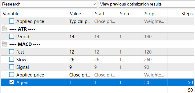
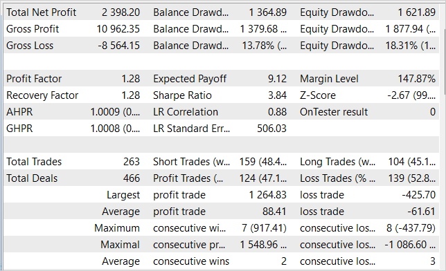
While training the models, we managed to obtain an Actor policy capable of generating profit on the training sample and generalizing the acquired knowledge for subsequent environmental states. For example, in the strategy tester, the model we trained was able to generate a profit of 23.98% within a month following the training sample. During the testing period, the model performed 263 trading operations, 47% of which were closed with a profit. The maximum profit per trade is almost 3 times higher than the maximum losing trade. The average profit per trade is 44% higher than the average loss. All this together allowed us to obtain a profit factor of 1.28. The graph shows a clear upward trend in the balance line.

Conclusion
The article considered the Stochastic Marginal Actor-Critic method offering an innovative approach to solving reinforcement learning problems. Based on the principle of maximum entropy, SMAC allows the agent to explore the environment more efficiently and learn more robustly, which is achieved by introducing an additional stochastic latent variable node.
The use of latent variables in the Agent's policy significantly increases its expressiveness and ability to model stochasticity in observations and rewards.
However, there are some difficulties in training policies with latent variables. The method authors offer solutions to cope with these difficulties.
In the practical part, we successfully integrated SMAC into the NNM method architecture, creating a simple and effective policy optimization method, as verified by testing results. We were able to train the Actor policy capable of generating returns of up to 24% per month.
Considering these results, the SMAC method is an effective solution for solving practical problems.
However, keep in mind that all the programs presented in the article were created only to demonstrate the method and are not suitable for working on real accounts. They require additional functionality configuration and optimization.
Let me remind you that financial markets are a high-risk type of investment. All risks from transactions performed by you or your electronic trading tools are entirely your responsibility.
Links
- Latent State Marginalization as a Low-cost Approach for Improving Exploration
- Neural networks made easy (Part 56): Using nuclear norm to drive research
Programs used in the article
| # | Name | Type | Description |
|---|---|---|---|
| 1 | Research.mq5 | Expert Advisor | Example collection EA |
| 2 | Study.mq5 | Expert Advisor | Agent training EA |
| 3 | Test.mq5 | Expert Advisor | Model testing EA |
| 4 | Trajectory.mqh | Class library | System state description structure |
| 5 | NeuroNet.mqh | Class library | A library of classes for creating a neural network |
| 6 | NeuroNet.cl | Code Base | OpenCL program code library |
Translated from Russian by MetaQuotes Ltd.
Original article: https://www.mql5.com/ru/articles/13290
Warning: All rights to these materials are reserved by MetaQuotes Ltd. Copying or reprinting of these materials in whole or in part is prohibited.
This article was written by a user of the site and reflects their personal views. MetaQuotes Ltd is not responsible for the accuracy of the information presented, nor for any consequences resulting from the use of the solutions, strategies or recommendations described.

 Deep Learning Forecast and ordering with Python and MetaTrader5 python package and ONNX model file
- Free trading apps
- Over 8,000 signals for copying
- Economic news for exploring financial markets
You agree to website policy and terms of use
Every pass of the Test EA generates drastically different results as if the modell were different from all previous ones. It is obvious that the model evolves every single pass of Test but the behaviour of this EA is hardly an evolution, so what stands behind it?
Here are some pictures:
This model use stochastic politic of Actor. So in the beginning of study we can see random deals at every pass. We collect this passes and restart study of the model. And repeat this process some times. While Actor find good politic of actions.
Let's put the question another way. Having collected (Research) samples and processed them (Study) we run the Test script. In several conscutive runs, without any Research or Study, the results obtained are completely different.
Test script loads a trained model in OnInit subroutine (line 99). Here we feed the EA with a model which should not change during Test processing. It should be stable, as far as I understand. Then, final results should not change.
In the meantime, we do not conduct any model training. Only collecting more samples is performed by the Test.
Randomness is rather observed in the Research module and possibly in the Study while optimizing a policy.
Actor is invoked in line 240 in order to calculate feedforward results. If it isn't randomly initialized at the creation moment, I believe this is the case, it should not behave randomly.
Do you find any misconception in the reasoning above?
The Actor use stochastic policy. We implement it by VAE.
Layer CNeuronVAEOCL use data of previous layer as mean and STD of Gaussian distribution and sample same action from this distribution. At start we put in model random weights. So it generate random means and STDs. At final we have random actions at every pass of model test. At time of study model will find some means for every state and STD tends to zero.