
Neural networks made easy (Part 48): Methods for reducing overestimation of Q-function values

Introduction
In the previous article, I considered the Deep Deterministic Policy Gradient (DDPG) method designed for training models in a continuous action space. This allows us to raise our model training to the next level. As a result, our last Agent is capable of not only predicting the upcoming direction of price movement, but also performs capital and risk management functions. It indicates the optimal size of the position to be opened, as well as stop loss and take profit levels.
However, DDPG has its drawbacks. Like other followers of Q-learning, it is subject to the problem of overestimating the values of the Q-function. During training, the error can accumulate, which ultimately leads to the agent learning a suboptimal strategy.
As you might remember, in DDPG, the Critic model learns the Q-function (prediction of expected reward) based on the results of interaction with the environment, while the Agent model is trained to maximize the expected reward, based only on the results of the Critic’s assessment of actions. Consequently, the quality of the Critic’s training greatly influences the Agent’s behavioral strategy and its ability to make optimal decisions.
1. Approaches to reducing overvaluation
The problem of overestimating the Q-function values appears quite often when training various models using the DQN method and its derivatives. It is characteristic of both models with discrete actions and when solving problems in a continuous space of actions. The causes of this phenomenon and methods of combating its consequences may be specific in each individual case. Therefore, an integrated approach to solving this problem is important. One such approach was presented in the article "Addressing Function Approximation Error in Actor-Critic Methods" published in February 2018. It proposed the algorithm called Twin Delayed Deep Deterministic policy gradient (TD3). The algorithm is a logical continuation of DDPG and introduces some improvements to it that boosts the quality of model training.
First, the authors add a second Critic. The idea is not new and has previously been used for discrete action space models. However, the authors of the method contributed their understanding, vision and approach to the use of the second Critic.
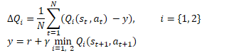
The idea is that both Critics are initialized with random parameters and trained in parallel on the same data. Initialized with different initial parameters, they begin their training from different states. But both Critics are trained on the same data, therefore they should move towards the same (desirably global) minimum. It is quite natural that during training the results of their forecasts will converge. However, they will not be identical due to the influence of various factors. Each of them is subject to the problem of overestimating the Q-function. But at a single point in time, one model will overestimate the Q-function, while the second one will underestimate it. Even when both models overestimate the Q-function, the error of one model will be less than that of the second one. Based on these assumptions, the method authors propose to use the minimal prediction to train both Critics. Thus, we minimize the impact of overestimation of the Q-function and the accumulation of errors during the learning process.
Mathematically, this method can be represented as follows:
Similar to DDPG, the authors of TD3 recommend using soft updating of target models. Using practical examples, the authors demonstrate that using soft updating of target models leads to a more stable Q-function learning process with less variance in results. At the same time, the use of more stable (less updated) goals in training process leads to a decrease in the accumulation of the Q-function re-assessment error.
The results of the experiments prompted the method authors to update the Actor policy more rarely.
As you know, training neural networks is an iterative process of gradually reducing errors. Training speed is determined by the training coefficients and the parameter updating algorithm. This approach allows averaging the error on the training sample and build a model as close as possible to the process being studied.
The results of the Actor model are part of the critic's training set. A rare update of the Actor policy allows us to reduce the stochasticity of the Critic training sample and, thereby, increase the stability of its training.
In turn, training the Actor using data from evaluating the results of a more accurate Critic allows us to improve the quality of the Actor work and eliminate unnecessary update operations with erroneous results.
Additionally, the authors of the TD3 algorithm proposed adding smoothing of the objective function to the training process. Using the subprocess is based on the assumption that similar actions lead to similar results. We assume that performing two slightly different actions will lead to the same result. Therefore, adding minor noise to the Agent's actions will not change the reward from the environment. But this will allow us to add some stochasticity to the Critic’s learning process and smooth out its assessments in a certain environment of target values.
![]()
This method allows introducing a kind of regularization into the Critic’s training and smooth out peaks leading to an overestimation of the Q-function values.
Thus, Twin Delayed Deep Deterministic policy gradient (TD3) introduces 3 main additions to the DDPG algorithm:
- Parallel training of 2 Critics
- Delay for updating Actor parameters
- Smoothing the target function.
As you can see, all 3 additions relate only to the arrangement of training and do not affect the architecture of the models.
2. Implementation using MQL5
In the practical part of the article, we will consider the implementation of the TD3 algorithm using MQL5. In this implementation, we use only 2 of the 3 additions. I did not add smoothing of the objective function due to the stochasticity of the financial market itself. We are unlikely to find 2 completely identical states in the entire training set.
We also return to the experience of using 3 EAs:
- Research — collecting examples database
- Study — model training
- Test — checking obtained results.
In addition, we are making changes to the interpretation of the model results, as well as to the EA’s trading algorithm.
2.1. Change in trading algorithm
First, let's talk about changing the trading algorithm. I decided to move away from the endless opening of new positions using the "open and forget" principle (a position is opened based on the results of an analysis of the current market situation, and closed according to a stop loss or take profit). Instead, we will open and maintain a position. At the same time, we do not exclude additions and partial closure of the position.
In this paradigm, we change the interpretation of the model signals. As before, the Agent returns 6 values: position size, stop loss and take profit in 2 trading directions. But now we will compare the received volume with the current position and, if necessary, add or partially close the position. We will add funds using standard means. In order to partially close positions, we will create the ClosePartial function.
We can close part of one position using standard means. But we assume the presence of several positions opened as a result of top-ups. Therefore, the task of the created function is to close positions using the FIFO (First In - First Out) method for the total volume.
In the parameters, the function receives the position type and closing volume. In the function body, we immediately check the received volume of closing positions and, if an incorrect value is received, we terminate the function.
Next, we arrange a cycle of searching through all open positions. In the loop body, check the instrument and type of the open position. When finding the required position, we check its volume. Here there are 2 options:
- the position volume is less than or equal to the closing volume - we close the position completely, and reduce the closing volume by the position volume
- the position volume is greater than the closing volume - we partially close the position and reset the closing volume to zero.
We carry out iterations of the cycle until all open positions are searched or until the volume to close is greater than "0".
bool ClosePartial(ENUM_POSITION_TYPE type, double value)
  {
   if(value <= 0)
      return true;
//---
   for(int i = 0; (i < PositionsTotal() && value > 0); i++)
     {
      if(PositionGetSymbol(i) != Symb.Name())
         continue;
      if(PositionGetInteger(POSITION_TYPE) != type)
         continue;
      double pvalue = PositionGetDouble(POSITION_VOLUME);
      if(pvalue <= value)
        {
         if(Trade.PositionClose(PositionGetInteger(POSITION_TICKET)))
           {
            value -= pvalue;
            i--;
           }
        }
      else
        {
         if(Trade.PositionClosePartial(PositionGetInteger(POSITION_TICKET), value))
            value = 0;
        }
     }
//---
   return (value <= 0);
  }
We have decided on the position size. Now let's talk about stop loss and take profit levels. From trading experience, we know that when the price moves against a position, shifting the stop loss level is bad practice, which only causes increased risks and loss accumulation. Therefore, we will trail the stop loss only in the direction of a trade. We allow the take profit level to be moved in both directions. The logic here is simple. We could have initially set the take profit more conservatively, but market developments suggest a stronger movement. Therefore, we can trail the stop loss and still raise the expected profit bar. If we miss the expected market movement, we can lower the profitability bar. We take only what the market gives.
To implement the described functionality, we create the TrailPosition function. In the function parameters, we specify the position type, stop loss and take profit prices. Please note that we indicate exactly the prices of trading levels, and not indents in points from the current price.
We do not check the specified levels in the function body. We will leave this up to the user and make a note about the need for such control on the side of the main program.
Next, we arrange a cycle of searching through all open positions. Similar to the function of partially closing a position, in the body of the loop we check the instrument and type of the open position.
When we find the desired position, we save the current stop loss and take profit of the position into local variables. At the same time, we set the position modification flag to 'false'.
After this, we check the deviation of the trading levels of the open position from those obtained in the parameters. Checking the need for modification depends on the type of open position. Therefore, we carry out this control in the body of the 'switch' statement with a check of the position type. If it is necessary to change at least one of the trading levels, we replace the corresponding value in the local variable and change the position modification flag to 'true'.
At the end of the loop operations, we check the value of the position modification flag and update its trading levels if necessary. The result of the operation is stored in a local variable.
After searching through all open positions, we complete the function returning the logical result of the performed operations to the calling program.
bool TrailPosition(ENUM_POSITION_TYPE type, double sl, double tp)
  {
   int total = PositionsTotal();
   bool result = true;
//---
   for(int i = 0; i <total; i++)
     {
      if(PositionGetSymbol(i) != Symb.Name())
         continue;
      if(PositionGetInteger(POSITION_TYPE) != type)
         continue;
      bool modify = false;
      double psl = PositionGetDouble(POSITION_SL);
      double ptp = PositionGetDouble(POSITION_TP);
      switch(type)
        {
         case POSITION_TYPE_BUY:
            if((sl - psl) >= Symb.Point())
              {
               psl = sl;
               modify = true;
              }
            if(MathAbs(tp - ptp) >= Symb.Point())
              {
               ptp = tp;
               modify = true;
              }
            break;
         case POSITION_TYPE_SELL:
            if((psl - sl) >= Symb.Point())
              {
               psl = sl;
               modify = true;
              }
            if(MathAbs(tp - ptp) >= Symb.Point())
              {
               ptp = tp;
               modify = true;
              }
            break;
        }
      if(modify)
         result = (Trade.PositionModify(PositionGetInteger(POSITION_TICKET), psl, ptp) && result);
     }
//---
   return result;
  }
Speaking about changes in the interpretation of the Actor's signals, it is worth paying attention to one more point. Previously, we used LReLU as the activation function on the actor's output. This allows us to get unlimited results in the upper values. It also allows us to display a negative result, which we regarded as a no deal signal. In the paradigm of the current interpretation of Actor signals, we decided to change the activation function to a sigmoid with the range from 0 to 1. As a trade volume, we are quite satisfied with these values. The same cannot be said about trading levels. In order to decipher the values of trading levels, we introduce 2 constants that determine the maximum size of the stop loss and take profit indentation from the price. By multiplying these constants by the corresponding Actor data, we will obtain trading levels in points from the current price.
#define                    MaxSL          1000
#define                    MaxTP          1000
In all other aspects, the architecture of our models remained the same. Therefore, I will not describe it here. You can find it in the attachment. As always, the description of the model architecture is located in "TD3\Trajectory.mqh", the CreateDescriptions function.
2.2. Building example database collecting EA
Now that we have decided on the principles of deciphering Actor signals and the basics of the trading algorithm, we can begin working directly on our model training EAs.
First, we will create the "TD3\Research.mq5" EA to collect a training sample of examples. The EA is built on the basis of previously reviewed similar EAs. In this article, we will only consider the OnTick method, which implements the trading algorithm described above. Otherwise, the new EA version is not much different from the previous ones.
At the beginning of the method, as before, we check the new candle opening event. Then we download the historical data of the symbol price movement and the parameters of the analyzed indicators.
void OnTick()
  {
//---
   if(!IsNewBar())
      return;
//---
   int bars = CopyRates(Symb.Name(), TimeFrame, iTime(Symb.Name(), TimeFrame, 1), HistoryBars, Rates);
   if(!ArraySetAsSeries(Rates, true))
      return;
//---
   RSI.Refresh();
   CCI.Refresh();
   ATR.Refresh();
   MACD.Refresh();
   Symb.Refresh();
   Symb.RefreshRates();
We pass the downloaded data to a buffer describing the current state of the environment.
   MqlDateTime sTime;
   float atr = 0;
   State.Clear();
   for(int b = 0; b < (int)HistoryBars; b++)
     {
      float open = (float)Rates[b].open;
      TimeToStruct(Rates[b].time, sTime);
      float rsi = (float)RSI.Main(b);
      float cci = (float)CCI.Main(b);
      atr = (float)ATR.Main(b);
      float macd = (float)MACD.Main(b);
      float sign = (float)MACD.Signal(b);
      if(rsi == EMPTY_VALUE || cci == EMPTY_VALUE || atr == EMPTY_VALUE || macd == EMPTY_VALUE || sign == EMPTY_VALUE)
         continue;
      //---
      State.Add((float)Rates[b].close - open);
      State.Add((float)Rates[b].high - open);
      State.Add((float)Rates[b].low - open);
      State.Add((float)Rates[b].tick_volume / 1000.0f);
      State.Add((float)sTime.hour);
      State.Add((float)sTime.day_of_week);
      State.Add((float)sTime.mon);
      State.Add(rsi);
      State.Add(cci);
      State.Add(atr);
      State.Add(macd);
      State.Add(sign);
     }
The next step is to prepare a vector describing the account state.
   sState.account[0] = (float)AccountInfoDouble(ACCOUNT_BALANCE);
   sState.account[1] = (float)AccountInfoDouble(ACCOUNT_EQUITY);
//---
   double buy_value = 0, sell_value = 0, buy_profit = 0, sell_profit = 0;
   double position_discount = 0;
   double multiplyer = 1.0 / (60.0 * 60.0 * 10.0);
   int total = PositionsTotal();
   datetime current = TimeCurrent();
   for(int i = 0; i < total; i++)
     {
      if(PositionGetSymbol(i) != Symb.Name())
         continue;
      double profit = PositionGetDouble(POSITION_PROFIT);
      switch((int)PositionGetInteger(POSITION_TYPE))
        {
         case POSITION_TYPE_BUY:
            buy_value += PositionGetDouble(POSITION_VOLUME);
            buy_profit += profit;
            break;
         case POSITION_TYPE_SELL:
            sell_value += PositionGetDouble(POSITION_VOLUME);
            sell_profit += profit;
            break;
        }
      position_discount += profit - (current - PositionGetInteger(POSITION_TIME)) * multiplyer * MathAbs(profit);
     }
   sState.account[2] = (float)buy_value;
   sState.account[3] = (float)sell_value;
   sState.account[4] = (float)buy_profit;
   sState.account[5] = (float)sell_profit;
   sState.account[6] = (float)position_discount;
//---
   Account.Clear();
   Account.Add((float)((sState.account[0] - PrevBalance) / PrevBalance));
   Account.Add((float)(sState.account[1] / PrevBalance));
   Account.Add((float)((sState.account[1] - PrevEquity) / PrevEquity));
   Account.Add(sState.account[2]);
   Account.Add(sState.account[3]);
   Account.Add((float)(sState.account[4] / PrevBalance));
   Account.Add((float)(sState.account[5] / PrevBalance));
   Account.Add((float)(sState.account[6] / PrevBalance));
As we can see, the preparation of initial data is similar to its arrangement in the previously discussed advisors.
Next, we transfer the prepared data to the input of the Actor model and perform a forward pass.
   if(Account.GetIndex() >= 0)
      if(!Account.BufferWrite())
         return;
//---
   if(!Actor.feedForward(GetPointer(State), 1, false, GetPointer(Account)))
      return;
Save the data we need on the next bar and get the result of the Actor’s work.
   PrevBalance = sState.account[0];
   PrevEquity = sState.account[1];
//---
   vector<float> temp;
   Actor.getResults(temp);
   float delta = MathAbs(ActorResult - temp).Sum();
   ActorResult = temp;
Please note that we only use the Actor model in this EA. After all, it is the Actor who generates the action in accordance with the learned policy (strategy). We will use Critic models while training the model.
Next, in order to maximize the study of the environment, we will add a little noise to the results of the Actor.
Here we need to remember that we have 2 modes for launching the EA. At the initial stage, we launch the EA without a pre-trained model and initialize our Actor with random parameters. In this mode, we do not need to add noise to explore the environment. After all, an untrained model will give chaotic values even without the noise. But when loading a pre-trained model, adding noise allows us to explore the environment in the vicinity of the Actor's decisions.
We limit the obtained values to the range of acceptable values of the sigmoid, which we use as the activation function at the output of the Actor model.
   if(AddSmooth)
     {
      int err = 0;
      for(ulong i = 0; i < temp.Size(); i++)
         temp[i] += (float)(temp[i] * Math::MathRandomNormal(0, 0.3, err));
      temp.Clip(0.0f, 1.0f);
     }
Next, we move on to the stage of decrypting the Actor’s results vector. First, we will save the main constants in local variables: the minimum position volume, the step of changing the position volume and the minimum indents of trading levels.
   double min_lot = Symb.LotsMin();
   double step_lot = Symb.LotsStep();
   double stops = MathMax(Symb.StopsLevel(), 1) * Symb.Point();
First, we decrypt the indicators of long positions. The first element of the vector is identified with the position volume. It should be greater than or equal to the minimum position volume. The second and third elements indicate the take profit and stop loss values, respectively. Let's adjust these elements by the maximum take profit and stop loss constants, and also multiply by the value of a single symbol point. As a result, we should get a value greater than the minimum indentation of trading levels. If at least one parameter does not meet the conditions, we close all open positions in this direction.
//--- buy control
   if(temp[0] < min_lot || (temp[1] * MaxTP * Symb.Point()) <= stops || (temp[2] * MaxSL * Symb.Point()) <= stops)
     {
      if(buy_value > 0)
         CloseByDirection(POSITION_TYPE_BUY);
     }
When the Actor's results recommend that we open or hold a long position, we normalize the position size in accordance with the broker's requirements for the analyzed symbol. Let's convert trading levels into specific price values. Then we call the above-described function for modifying open positions, indicating the POSITION_TYPE_BUY position type and the resulting price values of trading levels.
   else
     {
      double buy_lot = min_lot+MathRound((double)(temp[0]-min_lot) / step_lot) * step_lot;
      double buy_tp = NormalizeDouble(Symb.Ask() + temp[1] * MaxTP * Symb.Point(), Symb.Digits());
      double buy_sl = NormalizeDouble(Symb.Ask() - temp[2] * MaxSL * Symb.Point(), Symb.Digits());
      if(buy_value > 0)
         TrailPosition(POSITION_TYPE_BUY, buy_sl, buy_tp);
Next, we align the size of open positions with the Actor’s recommendations. If the volume of open positions is greater than recommended, then we call the function of partially closing positions. In the parameters of this function, we specify the POSITION_TYPE_BUY position type and the difference between open and recommended volumes as the size of positions to be closed.
If adding is recommended, then we open an additional position for the missing volume. At the same time, we indicate the recommended stop loss and take profit levels.
      if(buy_value != buy_lot)
        {
         if(buy_value > buy_lot)
            ClosePartial(POSITION_TYPE_BUY, buy_value - buy_lot);
         else
            Trade.Buy(buy_lot - buy_value, Symb.Name(), Symb.Ask(), buy_sl, buy_tp);
        }
     }
The parameters of a short position are decrypted in a similar way.
//--- sell control
   if(temp[3] < min_lot || (temp[4] * MaxTP * Symb.Point()) <= stops || (temp[5] * MaxSL * Symb.Point()) <= stops)
     {
      if(sell_value > 0)
         CloseByDirection(POSITION_TYPE_SELL);
     }
   else
     {
      double sell_lot = min_lot+MathRound((double)(temp[3]-min_lot) / step_lot) * step_lot;;
      double sell_tp = NormalizeDouble(Symb.Bid() - temp[4] * MaxTP * Symb.Point(), Symb.Digits());
      double sell_sl = NormalizeDouble(Symb.Bid() + temp[5] * MaxSL * Symb.Point(), Symb.Digits());
      if(sell_value > 0)
         TrailPosition(POSITION_TYPE_SELL, sell_sl, sell_tp);
      if(sell_value != sell_lot)
        {
         if(sell_value > sell_lot)
            ClosePartial(POSITION_TYPE_SELL, sell_value - sell_lot);
         else
            Trade.Sell(sell_lot - sell_value, Symb.Name(), Symb.Bid(), sell_sl, sell_tp);
        }
     }
At the end of the method, we add data to the trajectory array for subsequent saving it to the example database. Here we first generate a reward from the environment. As a reward, we use the relative change in balance, which we previously recorded in the first element of the vector describing the account state. If necessary, we add a penalty for the lack of open positions to this reward.
We add vectors of the current state of the environment and the results of the Actor to the state description structure. We entered the account status description data earlier. Call the method of adding the current state to the trajectory array.
//---
   float reward = Account[0];
   if((buy_value + sell_value) == 0)
      reward -= (float)(atr / PrevBalance);
   for(ulong i = 0; i < temp.Size(); i++)
      sState.action[i] = temp[i];
   State.GetData(sState.state);
   if(!Base.Add(sState, reward))
      ExpertRemove();
  }
Other EA functions were transferred with virtually no changes. You can find them in the attachment. We are moving on to the next stage of our work.
2.3. Creating a model training EA
The model is trained in the "TD3\Study.mq5" EA. In this EA, we arrange the entire TD3 algorithm with training of the Actor and 2 Critics.
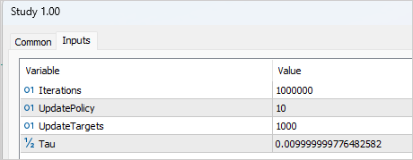
Arranging the training process requires adding several external variables that will help us manage training. As usual, here we indicate the number of iterations for updating the model parameters. In the context of the TD3 method, this refers to training Critic models.
input int Iterations = 1000000;
To indicate the frequency of Actor updates, we will create the UpdatePolicy variable, in which we will indicate how many Critic updates account for 1 Actor update.
input int UpdatePolicy = 3;
In addition, we will specify the update frequency of the target models and the update ratio.
input int                  UpdateTargets  = 100;
input float                Tau            = 0.01f;
In the global variables area, we will declare 6 instances of the neural network class: Actor, 2 Critics and target models.
CNet                 Actor;
CNet                 Critic1;
CNet                 Critic2;
CNet                 TargetActor;
CNet                 TargetCritic1;
CNet                 TargetCritic2;
The method of initializing the EA is almost identical to similar EAs from previous articles taking into account the different number of trained models. You can find it in the attachment.
But in the deinitialization method, we update and save the target models, not the trained ones (as was done previously). Target models are more static and less error prone.
void OnDeinit(const int reason)
  {
//---
   TargetActor.WeightsUpdate(GetPointer(Actor), Tau);
   TargetCritic1.WeightsUpdate(GetPointer(Critic1), Tau);
   TargetCritic2.WeightsUpdate(GetPointer(Critic2), Tau);
   TargetActor.Save(FileName + "Act.nnw", 0, 0, 0, TimeCurrent(), true);
   TargetCritic1.Save(FileName + "Crt1.nnw", TargetCritic1.getRecentAverageError(), 0, 0, TimeCurrent(), true);
   TargetCritic1.Save(FileName + "Crt2.nnw", TargetCritic2.getRecentAverageError(), 0, 0, TimeCurrent(), true);
   delete Result;
  }
Model training is arranged in the Train function. In the function body, save the number of loaded trajectories of the training sample into a local variable and arrange the training cycle according to the number of iterations specified in the external parameter.
void Train(void)
  {
   int total_tr = ArraySize(Buffer);
   uint ticks = GetTickCount();
In the loop body, we randomly select a trajectory and a state from the selected trajectory.
   for(int iter = 0; (iter < Iterations && !IsStopped()); iter ++)
     {
      int tr = (int)((MathRand() / 32767.0) * (total_tr - 1));
      int i = (int)((MathRand() * MathRand() / MathPow(32767, 2)) * (Buffer[tr].Total - 2));
First, we perform a forward pass on the target models, which will allow us to obtain the predictive value of the subsequent state.
In theory, we could train the models without the target function. After all, we could determine the value of the subsequent state from the accumulated actual subsequent reward. This approach might be suitable if we were dealing with the final state of the environment. But we are training the model for financial markets, which are infinite over the foreseeable time horizon. So, similar states 1 or 3 months ago have the same value for us since we want to take advantage of this experience in the future. Therefore, a well-trained Critic model will make results comparable regardless of the history depth.
Let's get back to our EA. We transfer data from the example database to buffers describing the state of the environment and form a vector describing the state of the account. Please note that we take data not for the selected, but for the subsequent state.
      //--- Target
      State.AssignArray(Buffer[tr].States[i + 1].state);
      float PrevBalance = Buffer[tr].States[i].account[0];
      float PrevEquity = Buffer[tr].States[i].account[1];
      Account.Clear();
      Account.Add((Buffer[tr].States[i + 1].account[0] - PrevBalance) / PrevBalance);
      Account.Add(Buffer[tr].States[i + 1].account[1] / PrevBalance);
      Account.Add((Buffer[tr].States[i + 1].account[1] - PrevEquity) / PrevEquity);
      Account.Add(Buffer[tr].States[i + 1].account[2]);
      Account.Add(Buffer[tr].States[i + 1].account[3]);
      Account.Add(Buffer[tr].States[i + 1].account[4] / PrevBalance);
      Account.Add(Buffer[tr].States[i + 1].account[5] / PrevBalance);
      Account.Add(Buffer[tr].States[i + 1].account[6] / PrevBalance);
Then we arrange a direct pass through the target Actor model.
      if(Account.GetIndex() >= 0)
         Account.BufferWrite();
      if(!TargetActor.feedForward(GetPointer(State), 1, false, GetPointer(Account)))
        {
         PrintFormat("%s -> %d", __FUNCTION__, __LINE__);
         ExpertRemove();
         break;
        }
Next, we perform a direct pass of 2 target Critics models. The source data for both models is the target Actor model.
      if(!TargetCritic1.feedForward(GetPointer(TargetActor), LatentLayer, GetPointer(TargetActor)) ||
         !TargetCritic2.feedForward(GetPointer(TargetActor), LatentLayer, GetPointer(TargetActor)))
        {
         PrintFormat("%s -> %d", __FUNCTION__, __LINE__);
         ExpertRemove();
         break;
        }
The data obtained allows us to generate target values for training Critic models.
Let me remind you that each Critic returns only one value of the predicted action cost in the current conditions. Therefore, our target value will also be one number.
According to the TD3 algorithm, we take the minimum value from the 2 Target results of the Critics models. Multiply the resulting value by the discount factor and add the actual reward for the action taken from the example database.
      TargetCritic1.getResults(Result);
      float reward = Result[0];
      TargetCritic2.getResults(Result);
      reward = DiscFactor * MathMin(reward, Result[0]) + (Buffer[tr].Revards[i] - Buffer[tr].Revards[i + 1]);
At this point, we have a target value for the Critic. The TD3 algorithm provides only one target value for 2 Critic models. But before going back we need to make a forward pass of the Critics. There is a nuance here. As you know, the Critic architecture does not provide for a primary data processing unit. This functionality is performed by the Actor, and we transfer the latent state of the Actor to the Critic as the initial data for describing the state of the environment. Therefore, we first take the initial data from the example database and perform a forward pass through the Actor model.
      //--- Q-function study
      State.AssignArray(Buffer[tr].States[i].state);
      PrevBalance = Buffer[tr].States[MathMax(i - 1, 0)].account[0];
      PrevEquity = Buffer[tr].States[MathMax(i - 1, 0)].account[1];
      Account.Clear();
      Account.Add((Buffer[tr].States[i].account[0] - PrevBalance) / PrevBalance);
      Account.Add(Buffer[tr].States[i].account[1] / PrevBalance);
      Account.Add((Buffer[tr].States[i].account[1] - PrevEquity) / PrevEquity);
      Account.Add(Buffer[tr].States[i].account[2]);
      Account.Add(Buffer[tr].States[i].account[3]);
      Account.Add(Buffer[tr].States[i].account[4] / PrevBalance);
      Account.Add(Buffer[tr].States[i].account[5] / PrevBalance);
      Account.Add(Buffer[tr].States[i].account[6] / PrevBalance);
      //---
      if(Account.GetIndex() >= 0)
         Account.BufferWrite();
      //---
      if(!Actor.feedForward(GetPointer(State), 1, false, GetPointer(Account)))
        {
         PrintFormat("%s -> %d", __FUNCTION__, __LINE__);
         ExpertRemove();
         break;
        }
Here we should keep in mind that the Actor will most probably return actions that differ from the examples stored in the database in the process of training. However, the reward does not correspond to the stored action. Therefore, we unload the latent state of the Actor. Upload the perfect action from the example database. Using this data, we carry out a direct pass of both Critics.
      if(!Critic1.feedForward(Result,1,false, GetPointer(Actions)) ||
         !Critic2.feedForward(Result,1,false, GetPointer(Actions)))
        {
         PrintFormat("%s -> %d", __FUNCTION__, __LINE__);
         ExpertRemove();
         break;
        }
Here we should mind one more thing. In theory, we could save the latent state of the Actor at the stage of collecting the example database and now simply use the saved data. But the parameters of all neural layers change during the model training. Consequently, the data preprocessing block also changes while training the Actor. As a consequence, the latent representation of the same environmental state changes. If we train the Critic on incorrect initial data, we will end up with an unpredictable result when training the Actor. Of course, we want to avoid this. Therefore, to train Critics, we use a correct latent representation of the environment state along with completed actions from the example database and the corresponding reward.
Next, we fill the target value buffer and perform a reverse pass through both Critics.
      Result.Clear();
      Result.Add(reward);
      if(!Critic1.backProp(Result, GetPointer(Actions), GetPointer(Gradient)) ||
         !Critic2.backProp(Result, GetPointer(Actions), GetPointer(Gradient)))
        {
         PrintFormat("%s -> %d", __FUNCTION__, __LINE__);
         ExpertRemove();
         break;
        }
Let's move on to Actor training. As was said in the theoretical part of this article, Actor parameters are updated less frequently. Therefore, we first check the need for this procedure at the current iteration.
      //--- Policy study
      if(iter > 0 && (iter % UpdatePolicy) == 0)
        {
When the moment comes to update the Actor’s parameters, we randomly select new initial data in order to maintain objectivity.
         tr = (int)((MathRand() / 32767.0) * (total_tr - 1));
         i = (int)((MathRand() * MathRand() / MathPow(32767, 2)) * (Buffer[tr].Total - 2));
         State.AssignArray(Buffer[tr].States[i].state);
         PrevBalance = Buffer[tr].States[MathMax(i - 1, 0)].account[0];
         PrevEquity = Buffer[tr].States[MathMax(i - 1, 0)].account[1];
         Account.Clear();
         Account.Add((Buffer[tr].States[i].account[0] - PrevBalance) / PrevBalance);
         Account.Add(Buffer[tr].States[i].account[1] / PrevBalance);
         Account.Add((Buffer[tr].States[i].account[1] - PrevEquity) / PrevEquity);
         Account.Add(Buffer[tr].States[i].account[2]);
         Account.Add(Buffer[tr].States[i].account[3]);
         Account.Add(Buffer[tr].States[i].account[4] / PrevBalance);
         Account.Add(Buffer[tr].States[i].account[5] / PrevBalance);
         Account.Add(Buffer[tr].States[i].account[6] / PrevBalance);
Next, we carry out a forward Actor pass.
         if(Account.GetIndex() >= 0)
            Account.BufferWrite();
         //---
         if(!Actor.feedForward(GetPointer(State), 1, false, GetPointer(Account)))
           {
            PrintFormat("%s -> %d", __FUNCTION__, __LINE__);
            ExpertRemove();
            break;
           }
Then we carry out a forward pass of one Critic. Please note that we are not using data from the example database here. Critic forward pass is carried out entirely on the new results of the Actor since it is important for us to evaluate the current model policy.
         if(!Critic1.feedForward(GetPointer(Actor), LatentLayer, GetPointer(Actor)))
           {
            PrintFormat("%s -> %d", __FUNCTION__, __LINE__);
            ExpertRemove();
            break;
           }
To update the Actor parameters, I used Critic1. According to my observations, the choice of the Critic model in this case is not that important. Despite the difference in ratings, both Critics returned identical error gradient values to the Actor during the test.
Actor training is aimed at maximizing the expected reward. We take the current result of the Critic's assessment of actions and add a small positive constant to it. When receiving a negative assessment of the actions, I used my positive constant as the target value. In this way, I sought to speed up my exit from the area of negative assessments.
         Critic1.getResults(Result);
         float forecast = Result[0];
         Result.Update(0, (forecast > 0 ? forecast + PoliticAdjust : PoliticAdjust));
While updating the Actor parameters, the Critic model is used only as a kind of loss function. It only generates an error gradient at the Actor's output. In this case, the critic parameters do not change. For this purpose, we disable the Critic’s training mode before the reverse pass. After transferring the error gradient to the Actor, we return the Critic to the training mode.
         Critic1.TrainMode(false);
         if(!Critic1.backProp(Result, GetPointer(Actor)) ||
            !Actor.backPropGradient(GetPointer(Account), GetPointer(Gradient)))
           {
            Critic1.TrainMode(true);
            PrintFormat("%s -> %d", __FUNCTION__, __LINE__);
            ExpertRemove();
            break;
           }
         Critic1.TrainMode(true);
        }
After receiving the error gradient from the Critic, we perform a reverse pass of the Actor.
At this stage, we arranged the training of the Q-function by the Critics and teaching the policy to the Actors. All we have to do is implement a soft update of the target models. This was described in detail in the previous article. Here we just check when the models are updated and call the appropriate methods for each target model.
      //--- Update Target Nets
      if(iter > 0 && (iter % UpdateTargets) == 0)
        {
         TargetActor.WeightsUpdate(GetPointer(Actor), Tau);
         TargetCritic1.WeightsUpdate(GetPointer(Critic1), Tau);
         TargetCritic2.WeightsUpdate(GetPointer(Critic2), Tau);
        }
At the end of the loop iteration, we inform a user about training and display the current errors of both critics. We do not display indicators of the Actor training quality, since the error is not calculated for this model.
      if(GetTickCount() - ticks > 500)
        {
         string str = StringFormat("%-15s %5.2f%% -> Error %15.8f\n", "Critic1", iter * 100.0 / (double)(Iterations),
                                                                                    Critic1.getRecentAverageError());
         str += StringFormat("%-15s %5.2f%% -> Error %15.8f\n", "Critic2", iter * 100.0 / (double)(Iterations),
                                                                                    Critic2.getRecentAverageError());
         Comment(str);
         ticks = GetTickCount();
        }
     }
After completing the loop iterations, we clear the comment area and initiate the EA shutdown process.
   Comment("");
//---
   PrintFormat("%s -> %d -> %-15s %10.7f", __FUNCTION__, __LINE__, "Critic1", Critic1.getRecentAverageError());
   PrintFormat("%s -> %d -> %-15s %10.7f", __FUNCTION__, __LINE__, "Critic2", Critic2.getRecentAverageError());
   ExpertRemove();
//---
  }
We will not dwell on the description of the algorithm for testing the trained model "TD3\Test.mq5". Its code almost completely repeats the example database collection EA. I have only excluded the addition of noise to the results of the Actor's work since we want to evaluate the quality of the model’s training, which excludes the study of the environment. At the same time, I have left the block for collecting the trajectory and recording it in the example database. This will allow us to save successful and unsuccessful passes. This will subsequently allows us to do error correction during the next start of the training process.
Find the full code of all used programs in the attachment.
3. Test
Let's move on to training and testing the results obtained. As usual, the models were trained on historical data of EURUSD H1 from January–May 2023. The indicator parameters and all hyperparameters were set to their default values.
Training was quite prolonged and iterative. At the first stage, a database of 200 trajectories was created. The first training process was run for 1,000,000 iterations. The Actor's policy was updated once after every 10 iterations of updating the Critics' parameters. A soft update of the target models was carried out after every 1,000 iterations of the Critics' update.
After that, another 50 trajectories were added to the example database and the second stage of model training was launched. At the same time, the number of iterations before updating the Actor and target models was reduced to 3 and 100, respectively.
After approximately 5 training cycles (50 trajectories were added at each cycle), a model was obtained that was capable of generating profit on the training set. After 5 months of the training sample, the model was able to receive almost 10% of the income. This is not the greatest result. 58 transactions were made. The share of profitable ones approached a meager 40%. Profit factor - 1.05, recovery factor - 1.50. The profit was achieved due to the size of profitable positions. The average profit from one trade is 1.6 times the average loss. The maximum profit is 3.5 times the maximum loss from one trading operation.
It is noteworthy that the drawdown on the balance is almost 32%, while Equity barely exceeds 6%. As you can see on the chart, we observe drawdowns in the balance with a flat or even growing Equity curve. This effect is explained by the simultaneous opening of multidirectional positions. When the stop loss of a losing position is triggered, we observe a drawdown in the balance. At the same time, an open position in the opposite direction accumulates profit, which is reflected in the Equity curve.


As we remember, in the previous article, the model showed a more significant result on the training set, but could not repeat it on new data. Now the situation is reversed. We have not received excess profits on the training set, but the model has shown stable results outside the training set. When testing the model on subsequent data that is not included in the training set, we see a “smaller copy” of the previous test. The model received 2.5% profit in 1 month. Profit factor - 1.07, recovery factor - 1.16. Only 27% of profitable trades, but the average profitable trade is almost 3 times higher than the average losing trade. The drawdown of 32% in terms of the balance and only 2% in terms of the Equity.


Conclusion
In this article, we got acquainted with the Twin Delayed Deep Deterministic policy gradient (TD3) algorithm. The method authors propose several important improvements to the DDPG algorithm, which can increase the efficiency of the method and the stability of model training.
As part of the article, we implemented this method using MQL5 and tested it on historical data. During the training process, a model was obtained that was capable of generating profit not only on training data, but also using the experience gained on new data. It is worth noting that on the new data the model obtained results comparable to the results of the training set. The results are not exactly what we would like to get. There are things that still need to be worked on. But one thing is certain - the TD3 algorithm allows training a model that works reliably on new data.
Generally, we can use the algorithm for further research in building a model for real trading.
List of references
Programs used in the article
| # | Name | Type | Description |
|---|---|---|---|
| 1 | Research.mq5 | Expert Advisor | Example collection EA |
| 2 | Study.mq5 | Expert Advisor | Agent training EA |
| 3 | Test.mq5 | Expert Advisor | Model testing EA |
| 4 | Trajectory.mqh | Class library | System state description structure |
| 5 | NeuroNet.mqh | Class library | A library of classes for creating a neural network |
| 6 | NeuroNet.cl | Code Base | OpenCL program code library |
Translated from Russian by MetaQuotes Ltd.
Original article: https://www.mql5.com/ru/articles/12892
Warning: All rights to these materials are reserved by MetaQuotes Ltd. Copying or reprinting of these materials in whole or in part is prohibited.
This article was written by a user of the site and reflects their personal views. MetaQuotes Ltd is not responsible for the accuracy of the information presented, nor for any consequences resulting from the use of the solutions, strategies or recommendations described.

- Free trading apps
- Over 8,000 signals for copying
- Economic news for exploring financial markets
You agree to website policy and terms of use
Thank you Dimitry for this wonderful series!
When compiling Trajectory.mqh an error emerged on line number 274 "int total = ArraySize(Buffer);" and the error is 'Buffer - undeclared identifier". I was searching in your previous article but on this part (48) the function SaveTotalBase() is the first time it is mention on the sourcecode. have I missed something?
Hi, you don't need to compile Trajectory.mqh. It's just a library to use in other EA.