Category Theory (Part 9): Monoid-Actions

Introduction

In prior article we introduced monoids and saw how they could be used in supervised learning to classify and inform trading decisions. To continue we will explore monoid actions and how they can also be used in unsupervised learning to reduce dimensions on input data. Monoid outputs from their operations always result in members of their set, meaning they are not transformative. It is monoid actions therefore that add ability of transformation since action set does not have to be monoid set subset. By transformation we mean ability to have action outputs that are not members of monoid set.

Formally, monoid action a of monoid M (e, *) on a set S is defined as:

a: M x S - - > S ;                                (1)

e a s - - > s;                                      (2)

m * (n * s) - - > (m * n) a s                (3)

Where m, n are members of monoid M, and s is a member of set S.

Illustration and Methods

Understanding relative importance of different features in a model's decision-making process is valuable. In our case, as per prior article, our ‘features’ were:

• Lookback period
• Timeframe
• Applied Price
• Indicator
• And decision to range or trend.

We will look at a few techniques that are applicable to weight our model’s features and help identify most sensitive one to accuracy of our forecast. We will select one technique, and based on its recommendation we will look to add transformation to monoid at that node, by expanding monoid set, through monoid actions, and see what effect this has on our ability to accurately place trailing stops, as per the application we considered in the previous article.

When determining relative importance of each data column in a training set, there are several tools and methods that can be employed. These techniques help quantify contribution of each feature (data-column) to model's predictions and guide us on what data column perhaps needs to be elaborated and what should be paid less attention to. Here are some commonly used methods:

Feature Importance Ranking

This approach ranks features based on importance by considering impact on model performance. Usually various algorithms, such as Random Forests, Gradient Boosting Machines (GBMs), or Extra Trees, provide built-in feature importance measures that not only help in building trees, but can be extracted after model training.

To illustrate this let's consider a scenario where, as in previous article, we want to forecast changes in price range, and use this in adjusting trailing stop of open positions. We will therefore be considering decision points we had then (features or data-columns) as trees. If we use a Random Forest classifier for this task, by taking each of our decision points as a tree, after training model, we can extract feature importance ranking.

To clarify, our dataset will contain following trees:

• Length of look-back analysis period (integer data)
• Time frame chosen in trading (enumeration data: 1-hour, 2-hour, 3-hour, etc.)
• Applied price used in analysis (enumeration data: open-price, median-price, typical-price, close-price)
• Choice of indicator used in analysis (enumeration data of RSI oscillator or Bollinger Bands Envelopes)

After training with Random Forest classifier, we can extract feature importance ranking by with Gini impurity weights. Feature importance scores indicate relative importance (weighting) of each data column in model's decision-making process.

Let's assume feature importance ranking resulted in following:

• Choice of indicator used in analysis: 0.45
• Length of look-back analysis period: 0.30
• Applied price used in analysis: 0.20
• Time frame chosen in trading: 0.05

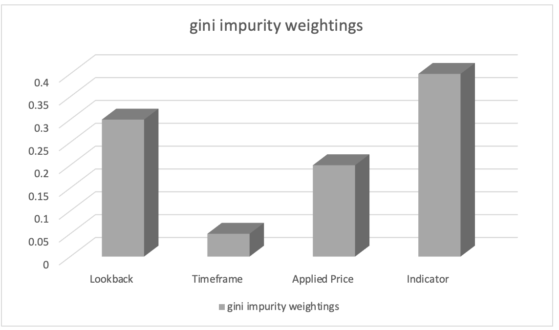
Based on this, we can infer that "Choice of indicator used in analysis" feature has highest importance, followed by "Length of look-back analysis period" feature. "Applied price used in analysis" feature is ranked third, while "Time frame chosen in trading" feature has least importance.

This information can guide us in understanding which features are most significant in impacting model's predictions and with this knowledge we would focus on more important features during feature engineering, prioritise feature selection, or explore further domain-specific insights related to these features. In our case we could look at transforming monoid set of indicators by introducing monoid-action set(s) of other indicators and examine how that influences our forecasts. So, our action sets would add alternative indicators to RSI oscillator and Bollinger Bands Envelope. Whichever indicator we add though, as was case with Bollinger Bands in previous article, we would need to regularise its output and ensure it is in range from 0 to 100 with 0 indicating decreasing price bar range while 100 indicates increasing range.

Permutation Importance

Permutation importance assesses significance of order of features (or data columns) by randomly permuting their order and measuring subsequent change in model performance when making forecasts. Remember order thus far has been lookback period, then timeframe, then applied price, then indicator and finally trade decision type. What would happen if we sequenced our decisions differently? We would have to go about this by permuting only one data column (feature) at a time. A larger drop in forecast accuracy for any one of these data columns, would indicate higher importance. This method is model-agnostic and can be applied to any machine learning algorithm.

To illustrate this let’s consider a scenario with our same dataset of five columns, as above and in previous article, and we want to forecast changes in price bar range. We decide to use a Gradient Boosting Classifier for this task. To assess significance of each data column using permutation importance, we essentially train our model. When training Gradient Boosting Classifier using monoid operator functions and identity settings we used for our prior article, our dataset will resemble this table below:

To train a gradient boost classifier using our dataset we can follow this 4 step-by-step guide:

Preprocess Data:

This step begins with converting our discrete data (i.e. enumerations; price chart timeframe, applied price, indicator choice, trade decision) into numerical representations using techniques such as one-hot encoding. You then split dataset into features (data-columns 1-5) and model forecasts plus actual values (data-columns 6-7).

Split Data: After pre-processing we then need to divide dataset into rows for training set and rows for test set. This allows you to evaluate model's performance on unseen data while using settings that have worked best on your training data. Typically, an 80-20 split is used, but you can adjust ratio based on size and characteristics of rows in your dataset. For data-columns used in this article I would recommend a 60-40 split.

Create Gradient Boost Classifier: You then include necessary libraries or implement required functions for gradient boost classification in C/MQL5. This means to include in expert initialisation function, created instances of gradient boost classifier model where you also specify hyper parameters like number of estimators, learning rate, and maximum depth.

Train Model: By iterating over training data and varying order of each data column during decision-making process, training set is used to train gradient boost classifier. Model results are then logged. To increase accuracy of forecasts for price bar range adjustments, you may also vary model's parameters, such as each monoids identity element or operation type (from list of operations used in previous article).

Evaluate System: Model would be tested on test data rows (40% separated at split) using best settings from training. This allows you to determine how well-trained model settings perform on untrained data. In doing so, you would be running through all data rows in out-of-sample data (test data rows) to assess model’s best settings ability to forecast changes in target price bar range. Results from test runs could then be evaluated using methods like F-score, etc.

You can also fine-tune Model if performance needs improvement, by changing gradient boost classifier's hyper parameters. To discover best hyper parameters, you would need to utilise methods like grid search and cross-validation. After developing a successful model, you may use it to make assumptions about new, unforeseen data by preprocessing and encoding categorical variables in new data to ensure they have same format as training data. With this you would then predict our price bar range changes for new data using trained model.

Note that gradient boost classification implementation in MQL5 can be difficult and time-consuming from scratch. So use of machine learning libraries written in C, like XGBoost or LightGBM, which offer effective gradient boosting implementations with C APIs is highly recommended.

Let's imagine, for illustration, that after permuting our data columns, we obtain following outcomes:

• When lookback period is switched, forecasting performance falls by 0.062.
• Timeframe for permutation leads to performance decrease of 0.048
• Applying permutation on applied price, results in performance loss of 0.027
• Performance drops by 0.014 for shuffling indicator data-column position.
• Performance loss after permuting trade decision leads to 0.009

These findings lead us to conclusion that "lookback period" has biggest significance in its position when predicting changes in price bar range, as permuting its values caused greatest reduction in model performance. Second most significant feature is "timeframe," which is followed by "applied price," "indicator," and finally "trade decision."

By quantifying effect of each data column on model's performance, this method enables us to determine their relative relevance. By assessing relative significance of each feature (data column), we are better able to choose features, engineer features, and perhaps even highlight areas in which our prediction model needs more research and development.

We might therefore propose monoid actions for lookback monoid set that alter it by adding additional lookback periods that are not already in monoid set in order to further explain improvement. This therefore enables us to investigate whether, if any, these additional periods have an impact on how well our model predicts changes in price bar range. Monoid set currently consists of values from 1 to 8, each of which is a multiple of 4. What if we our multiple was 3 or 2? What impact (if any) would this have on performance? Since we now understand lookback period's place in decision process and that it most sensitive to overall performance of system, these and comparable problems may be addressed.

SHAP Values

SHAP (SHapley Additive exPlanations) is a unified framework that assigns importance values to each data-column based on game theory principles. SHAP values provide a fair distribution of feature contributions, considering all possibilities. They offer a comprehensive understanding of feature importance in complex models like XGBoost, LightGBM, or deep learning models.

Recursive Feature Elimination (RFE)

RFE is an iterative feature selection method that works by recursively eliminating less important features based on their weights or importance scores. process continues until desired number of features is reached or a performance threshold is met. To illustrate this, we can use similar scenario above where we have a dataset of five columns from lookback period to trading decision type and we want to predict changes in price bar range based on each of 5 features (data-columns). We use a Support Vector Machine (SVM) classifier for this task. Here's how Recursive Feature Elimination (RFE) would thus be applied:

• Train Model with SVM classifier using all data-columns in dataset. Initially training is with everything.
• Ranking features happens next where we obtain weights or importance scores assigned to each feature by SVM classifier. These indicate relative importance of each in classification task.
• Elimination of least important feature is done next where we omit least important data-column based on SVM weights. This can be done by removing feature with lowest weight.
• Retraining model with reduced data-columns happens next, where SVM classifier is applied only remaining features.
• Performance evaluation without omitted data-column is done using an appropriate evaluation metric, such as accuracy or F-score.
• Process is repeated from Steps 2 to 5 until desired number of columns is arrived at through, eliminating least important feature(s) (or data-columns) in each iteration and retraining model with reduced feature set.

For instance, let's assume we start with five features and apply RFE and we have a target of 3 features. On Iteration 1 lets suppose this is ranking of features based on descending importance scores:

• Lookback period
• Timeframe
• Applied Price
• Indicator
• Trade Decision

Elimination of feature with lowest importance score, Trade Decision, would be done. Retraining SVM classifier with remaining features: Lookback, Timeframe, Applied Price, and Indicator would then follow. Lets take this to be the ranking on iteration 2:

• Lookback period
• Indicator
• Timeframe
• Applied Price

Eliminate feature with lowest importance score, this would be Applied Price. Since no more features are left to eliminate given that we’ve reached desired number of features iteration would halt. Iterative process stops as we have reached desired number of features (or another predefined stopping criterion like an F-Score threshold). Final model is therefore trained using selected features: Lookback period, Indicator, and Timeframe. RFE helps identify most important features for classification task by iteratively removing less relevant features. By selecting a subset of features that contribute most to model's performance, RFE can improve model efficiency, reduce overfitting, and enhance interpretability.

L1 Regularisation (Lasso)

L1 regularisation applies a penalty term to model's objective function, encouraging sparse feature weights. As a result, less important features tend to have zero or near-zero weights, allowing for feature selection based on magnitude of weights. Consider a scenario where a trader would like to gauge his exposure to real estate and REITs, and we have a dataset of housing prices, that we want to use predict price trend of residential houses based on various features such as area, number of bedrooms, number of bathrooms, location, and age. We can use L1 Regularisation, specifically Lasso algorithm, to assess importance of these features. Here's how it works:

• We start by training a linear regression model with L1 regularisation (Lasso) using all features in dataset. L1 regularisation term adds a penalty to model's objective function.
• After training Lasso model, we obtain estimated weights assigned to each feature. These weights represent importance of each feature in predicting housing prices. L1 regularisation encourages sparse feature  weights, meaning less important features tend to have zero or near-zero weights.
• Rank Features: We can rank features based on magnitude of weights. Features with higher absolute weights are considered more important, while features with close-to-zero weights are deemed less important.

For instance, if we assume we train a Lasso model on housing price dataset and obtain following feature weights:

• Area: 0.23
• Number of Bedrooms: 0.56
• Number of Bathrooms: 0.00
• Location: 0.42
• Age: 0.09

Based on these feature weights, we can rank features in terms of importance for predicting house prices:

• Number of Bedrooms: 0.56
• Location: 0.42
• Area: 0.23
• Age: 0.09
• Number of Bathrooms: 0.00

In this example, Number of Bedrooms has highest absolute weight, indicating its significance in predicting housing prices is high. Location and Area follow closely in importance, while Age has a relatively lower weight. Number of Bathrooms, in this case, has a weight of zero, suggesting it is deemed unimportant and has been effectively excluded from model.

By applying L1 regularisation (Lasso), we can identify and select most important features for predicting housing prices. regularisation penalty promotes sparsity in feature weights, allowing for feature selection based on magnitude of weights. This technique helps in understanding which features have most influence on target variable (residential price trend) and can be useful for feature engineering, model interpretation, and potentially improving model performance by reducing overfitting.

Principal Component Analysis (PCA)

PCA is a dimensionality reduction technique that can indirectly assess feature importance by transforming original features into a lower-dimensional space, PCA identifies directions of maximum variance. Principal components with highest variance can be considered more important.

Correlation Analysis

Correlation analysis examines linear relationship between features and target variable. Features with higher absolute correlation values are often considered more important for predicting target variable. However, it is important to note that correlation does not capture non-linear relationships.

Mutual Information

Mutual information measures statistical dependence between variables. It quantifies how much information on one variable can be obtained from another. Higher mutual information values indicate a stronger relationship and can be used to assess relative feature importance.

To illustrate we can consider a scenario where a trader/ investor is looking to open a position in an up and rising private equity startup based on a dataset of customer information, with goal to forecast customer churn based on various available features (our data-columns) such as age, gender, income, subscription type, and total purchases. We can use Mutual Information to assess importance of these. Here's how it would work:

• We start by calculating mutual information between each feature and target variable (customer churn). Mutual information measures amount of information that one variable contains about another variable. In our case, it quantifies how much information about customer churn can be obtained from each feature in our available data-columns.
• Once we have worked out mutual information scores, we rank these based on their values. Higher mutual information values indicate a stronger relationship between feature and customer churn, suggesting higher importance.

For example, if we assume mutual information scores for data-columns are:

• Age: 0.08
• Gender: 0.03
• Income: 0.12
• Subscription Type: 0.10
• Total Purchases: 0.15

Based on these, we can rank features in terms of their importance for predicting customer churn:

• Total Purchases: 0.15
• Income: 0.12
• Subscription Type: 0.10
• Age: 0.08
• Gender: 0.03

In this example, Total Purchases has highest mutual information score, indicating that it contains most information about customer churn. Income and Subscription Type follow closely, while Age and Gender have relatively lower mutual information scores.

By using Mutual Information, we are able to weight each data-column and explore which columns can be investigated further by adding monoid actions. This dataset is completely new not like what we had in prior article so to illustrate it is helpful to first construct monoids of each data column by defining respective sets. Total purchases of data column with supposedly highest mutual information, is continuous data and not discrete meaning we cannot augment monoid set as easily by introducing enumerations out of scope in base monoid. So, to study further or expand total purchases in monoid we could add dimension of purchase date. This means our action set will have continuous data of datetime. On pairing (via action) with monoid on total purchases, for each purchase we could get purchase date which would allow us explore significance of purchase dates and amounts on customer churn. This could lead to more accurate forecasts.

Model-Specific Techniques

Some machine learning algorithms have specific methods to determine feature importance. For instance, decision tree-based algorithms can provide feature importance scores based on number of times a feature is used to split data across different trees.

Let's consider a scenario where we have a dataset of customer information, and we want to predict whether a customer will purchase a product based on various features such as age, gender, income, and browsing history. We decide to use a Random Forest classifier for this task, which is a decision tree-based algorithm. Here's how we can determine feature importance using this classifier:

• We start by training a Random Forest classifier using all features in dataset. Random Forest is an ensemble algorithm that combines multiple decision trees.
• After training Random Forest model, we can extract feature importance scores specific to this algorithm. Feature importance scores indicate relative importance of each feature in classification task.
• We then rank features based on their importance scores. Features with higher scores are considered more important, as they have a greater impact on model’s performance.

For example, after training Random Forest classifier, we obtain following feature importance scores:

• Age: 0.28
• Gender: 0.12
• Income: 0.34
• Browsing History: 0.46

Based on these feature importance scores, we can rank features in terms of their importance for predicting customer purchases:

• Browsing History: 0.46
• Income: 0.34
• Age: 0.28
• Gender: 0.12

In this example, Browsing History has highest importance score, indicating that it is most influential feature in predicting customer purchases. Income follows closely, while Age and Gender have relatively lower importance scores. By leveraging specific methods of Random Forest algorithm, we can obtain feature importance scores based on number of times each feature is used to split data across different trees in ensemble. This information allows us to identify key features that contribute most significantly to prediction task. It helps in feature selection, understanding underlying patterns in data, and potentially improving model’s performance.

Expert Knowledge and Domain Understanding

In addition to quantitative methods, incorporating expert knowledge and domain understanding is crucial for assessing feature importance. Subject-matter experts can always provide insights into relevance and significance of specific features based on their expertise and experience. It is also important to note that different methods may yield slightly different results, and choice of technique may depend on specific characteristics of dataset and machine learning algorithm being used. It is often recommended to use multiple techniques to gain a comprehensive understanding of feature importance.

Implementation

To implement the weighting of our data-columns/ features we will use correlation. Since we are sticking with the same features we had in the previous article we will be comparing the correlation of the monoid set values to changes in price bar range to get the weighting of each data-column. Recall each data-column is a monoid with a set where the set values are the column values. Since we are testing, at the onset we do not know whether the most correlated column should be expanded (transformed by monoid actions) or it should be the data-column with the least correlation. To that end we will add an extra parameter that will help in making this selection across various test runs. And also we've introduced extra global parameters to cater for the monoid-actions.

//+------------------------------------------------------------------+
//|                                                   TrailingCT.mqh |
//|                   Copyright 2009-2013, MetaQuotes Software Corp. |
//|                                              http://www.mql5.com |
//+------------------------------------------------------------------+
#include <Math\Stat\Math.mqh>
#include <Expert\ExpertTrailing.mqh>
#include <ct_9.mqh>
// wizard description start
//+------------------------------------------------------------------+
//| Description of the class                                         |
//| Title=Trailing Stop based on 'Category Theory' monoid-action concepts  |
//| Type=Trailing                                                    |
//| Name=CategoryTheory                                              |
//| ShortName=CT                                                     |
//| Class=CTrailingCT                                                |
//| Page=trailing_ct                                                 |
//|....	
//| Parameter=IndicatorIdentity,int,0, Indicator Identity            |
//| Parameter=DecisionOperation,int,0, Decision Operation            |
//| Parameter=DecisionIdentity,int,0, Decision Identity              |
//| Parameter=CorrelationInverted,bool,false, Correlation Inverted   |
//+------------------------------------------------------------------+
// wizard description end
//+------------------------------------------------------------------+
//| Class CTrailingCT.                                               |
//| Appointment: Class traling stops with 'Category Theory'          |
//|               monoid-action concepts.                            |
//| Derives from class CExpertTrailing.                              |
//+------------------------------------------------------------------+
int                        __LOOKBACKS[8] = {1,2,3,4,5,6,7,8};
ENUM_TIMEFRAMES            __TIMEFRAMES[8] = {PERIOD_H1,PERIOD_H2,PERIOD_H3,PERIOD_H4,PERIOD_H6,PERIOD_H8,PERIOD_H12,PERIOD_D1};
ENUM_APPLIED_PRICE         __APPLIEDPRICES[4] = { PRICE_MEDIAN, PRICE_TYPICAL, PRICE_OPEN, PRICE_CLOSE };
string                     __INDICATORS[2] = { "RSI", "BOLLINGER_BANDS" };
string                     __DECISIONS[2] = { "TREND", "RANGE" };

#define                    __CORR 5
int                        __LOOKBACKS_A[10] = {1,2,3,4,5,6,7,8,9,10};
ENUM_TIMEFRAMES            __TIMEFRAMES_A[10] = {PERIOD_H1,PERIOD_H2,PERIOD_H3,PERIOD_H4,PERIOD_H6,PERIOD_H8,PERIOD_H12,PERIOD_D1,PERIOD_W1,PERIOD_MN1};
ENUM_APPLIED_PRICE         __APPLIEDPRICES_A[5] = { PRICE_MEDIAN, PRICE_TYPICAL, PRICE_OPEN, PRICE_CLOSE, PRICE_WEIGHTED };
//+------------------------------------------------------------------+
//|                                                                  |
//+------------------------------------------------------------------+
class CTrailingCT : public CExpertTrailing
  {
protected:
   //--- adjusted parameters
   double m_step;                // trailing step
   
   ...
   
   //
   
   CMonoidAction<double,double>  m_lookback_act;
   CMonoidAction<double,double>  m_timeframe_act;
   CMonoidAction<double,double>  m_appliedprice_act;
   
   bool                          m_correlation_inverted;
   
   int                           m_lookback_identity_act;
   int                           m_timeframe_identity_act;
   int                           m_appliedprice_identity_act;
   
   int                           m_source_size;       // Source Size

public:
   //--- methods of setting adjustable parameters
   
   
   
   
... 
   
   void                 CorrelationInverted(bool value)     { m_correlation_inverted=value;                 }
   
   
... 
   
  };

Also, the ‘Operate_X’ functions have been tidied up to just one function called ‘Operate’. In addition, the ‘Get’ functions for the data-columns have been expanded to accommodate monoid actions and an overload for each has been added to help with indexing respective global variable arrays.

This then is how we are developing our trailing class.

//+------------------------------------------------------------------+
//|                                                                  |
//+------------------------------------------------------------------+
void CTrailingCT::Operate(CMonoid<double> &M,EOperations &O,int &OutputIndex)
   {
      OutputIndex=-1;
      //
      double _values[];
      ArrayResize(_values,M.Cardinality());ArrayInitialize(_values,0.0);
      //

      
... 
      
      //
      
      if(O==OP_LEAST)
      {
         OutputIndex=0;
         double _least=_values[0];
         for(int i=0;i<M.Cardinality();i++)
         {
            if(_least>_values[i]){ _least=_values[i]; OutputIndex=i; }
         }
      }
      else if(O==OP_MOST)
      {
         OutputIndex=0;
         double _most=_values[0];
         for(int i=0;i<M.Cardinality();i++)
         {
            if(_most<_values[i]){ _most=_values[i]; OutputIndex=i; }
         }
      }
      else if(O==OP_CLOSEST)
      {
         double _mean=0.0;
         for(int i=0;i<M.Cardinality();i++)
         {
            _mean+=_values[i];
         }
         _mean/=M.Cardinality();
         
         OutputIndex=0;
         double _closest=fabs(_values[0]-_mean);
         for(int i=0;i<M.Cardinality();i++)
         {
            if(_closest>fabs(_values[i]-_mean)){ _closest=fabs(_values[i]-_mean); OutputIndex=i; }
         }
      }
      else if(O==OP_FURTHEST)
      {
         double _mean=0.0;
         for(int i=0;i<M.Cardinality();i++)
         {
            _mean+=_values[i];
         }
         _mean/=M.Cardinality();
         
         OutputIndex=0;
         double _furthest=fabs(_values[0]-_mean);
         for(int i=0;i<M.Cardinality();i++)
         {
            if(_furthest<fabs(_values[i]-_mean)){ _furthest=fabs(_values[i]-_mean); OutputIndex=i; }
         }
      }
   }
//+------------------------------------------------------------------+
//|                                                                  |
//+------------------------------------------------------------------+
int CTrailingCT::GetLookback(CMonoid<double> &M,int &L[])
   {
      m_close.Refresh(-1);
      
      int _x=StartIndex();
      
      
... 
   
      int _i_out=-1;
      //
      Operate(M,m_lookback_operation,_i_out);
      
      if(_i_out==-1){ return(4); }
      
      return(4*L[_i_out]);
   }
//+------------------------------------------------------------------+
//|                                                                  |
//+------------------------------------------------------------------+
ENUM_TIMEFRAMES CTrailingCT::GetTimeframe(CMonoid<double> &M, ENUM_TIMEFRAMES &T[])
   {
      
... 
      
      int _i_out=-1;
      //
      Operate(M,m_timeframe_operation,_i_out);
      
      if(_i_out==-1){ return(INVALID_HANDLE); }
      
      return(T[_i_out]);
   }

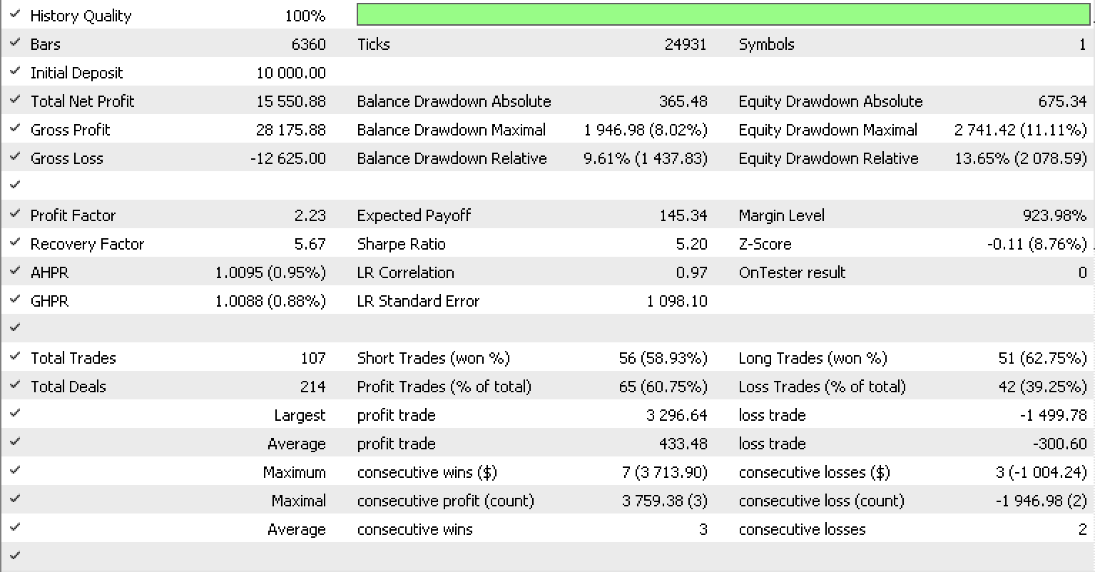
If we run tests as we did in the previous article for EURUSD on the on-hour timeframe from 2022.05.01 to 2023.05.15, using the library's inbuilt RSI signal class, this is our test report.

While the results from our report above are not as good as we had in best report in prior article they do highlight the sensitivity of report results to changes in our monoid sets, via monoid actions.

Conclusion

In summary we have looked at how transformed monoids aka monoid-actions can further fine tune a trailing stop system that makes forecasts on volatility in order to more accurately adjust the stop loss of open positions. This was looked at in tandem with various methods that are typically used in weighting model features (data-columns in our case), in order to better understand the model, its sensitivities, and which features if any need expansion to improve the model's accuracy. Hope you liked it and thanks for reading.