Cycles and trading

Introduction

The main task facing a trader is to predict price movements. Traders build their forecasts based on one model or another. One of the simplest and most visual models is the cyclical price movement model.

The basic idea behind any cyclical pattern is that various factors interact to create cycles in price movement. These cycles may differ from each other in their duration and strength. If you know the parameters of these cycles, then trading operations will become very simple: open a buy position when the cycle has reached its minimum, sell when the cycle has reached its maximum.

Let's see how this model can be used in practice.

Simple cycle

When describing cycles, we usually apply sine and cosine trigonometric functions. But the cycle can be defined in another way - with the help of finite differences.

For example, let's consider an equation in which the 2nd difference is proportional to the value of the time series:

This is a harmonic oscillator equation. At first glance, there is nothing special about it. But this equation has one interesting property. If the value of the R ratio lies in the range from 0 to 4, then this equation can only belong to a sinusoid. This ratio depends on the N cycle period. In other words, its value can be chosen such that the equation reacts only to cycles with a certain frequency:

Now let's see how this equation can be applied in practice. If we apply it to p[] prices, we will need the value of the m level the price fluctuates around.

To avoid calculating the value of this average level, I will resort to a little trick. Let's remember what happens mathematically when a cycle reaches a maximum or minimum point. At these moments, the 1st derivative changes sign.

Instead of the derivative, we will use the 1st difference of the original equation. This is the difficult fate of a trader - to look for differences from differences. But this approach greatly simplifies the calculations. We only need to set the value of the R ratio. The final form of the equation is as follows:

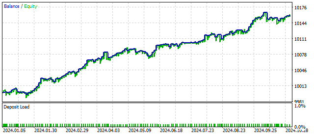
Further, I will call such equations trading algorithm equations. Based on this equation we can create a trading strategy. First, I will make a small addition - we can use any version of the conventional moving average instead of the current price. The essence of the strategy itself is very simple. Opening and closing positions occurs when the sign of the equation changes:

• from negative to positive - open buy, close sell;
• from positive to negative - open sell, close buy.

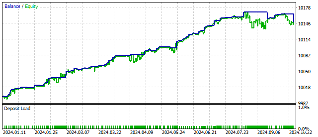
The EA balance change can be like this.

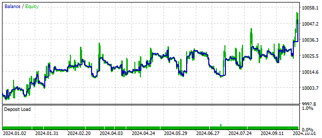
This trading strategy has prospects. But it needs some improvement.

Cycle with damping

The strategy we looked at earlier has one serious drawback. It is based on the assumption that the cycle will continue for quite a long time. In real life, the cycle depends on many external factors and can collapse almost immediately after it begins.

To get rid of this drawback, we can use the harmonic oscillator model with damping of oscillations. The equation of such a cycle is also set by finite differences:

The S parameter determines how quickly the oscillations die out. The higher its value, the faster the damping occurs. The critical value of this parameter can be found using the following equation:

Starting from this value, the oscillator's movement becomes non-oscillatory.

We already know what to do with such an equation. We need to find its 1st difference, which will generate trading signals.

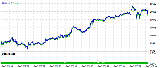
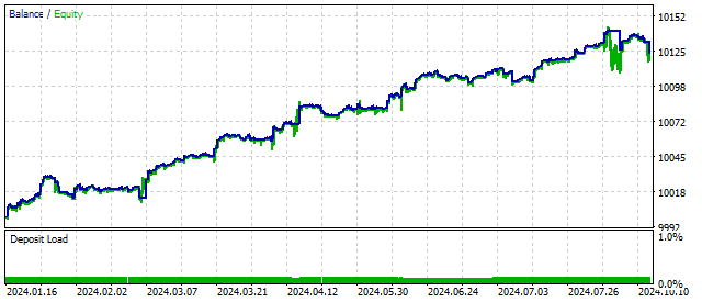
By adding a new parameter, the trading strategy may become more flexible and profitable. For example, this is what the balance change looks like at a critical value of S.

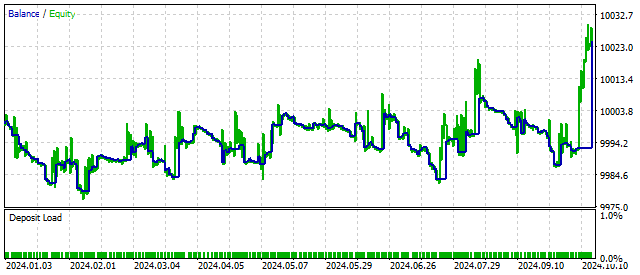
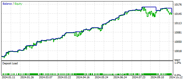
By definition, parameter S should be positive. But this requirement is not mandatory. If we set a negative value for this parameter, the original equation will describe oscillations with an ever-increasing amplitude. In this way, EA can react to the beginning of the cycle and possibly increase profitability. The trading results in this case may look like this:

As you can see, making the cycle model more complex can improve trading results. Let's try to complicate the model even more.

Elliott Waves

Elliott Wave Principle has been known for a very long time and is widely used in trading. Let's try to apply the cyclical model to Elliott waves.

The first five Elliott waves can be simulated as the sum of two sinusoids with different amplitudes and periods:

In this case, the following conditions should be met:

As a result, we can get something like this:

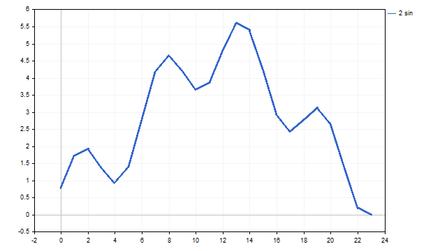
It does not look exactly like in the books - a little angular, but pretty similar.

We can simulate the sum of two sinusoids using finite differences:

where    — the value of the finite difference of order n, on the price reading with index i. We already know what to do with this equation - find the difference from the sum of the differences and get trading signals:

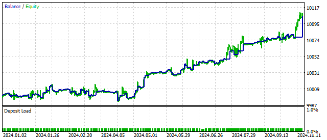
Using the sum of two sinusoids makes it possible to adjust the EA to more complex market situations. Using this trading algorithm can lead to both an increase in market entries and an improvement in their profitability.

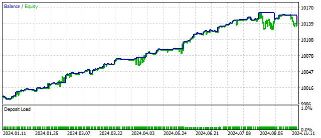
This is the result that an EA based on the Elliott wave principle can show:

As you can see, even a small complication of the cyclical model can bring positive results.

Generalized harmonic oscillator

We have already looked at three models based on the harmonic oscillator. Each of these models was built on its own initial assumptions. But as a result, we still got some sum of finite differences.

We can build a more general model. The essence of this model is very simple - first we take the difference of a predetermined order and add them to the differences of lower orders, down to the 1st one. In this case, each difference of low order is taken with its own weighting ratio.

For example, I took the difference of the 7th order. Then the equation for the trading algorithm will be as follows:

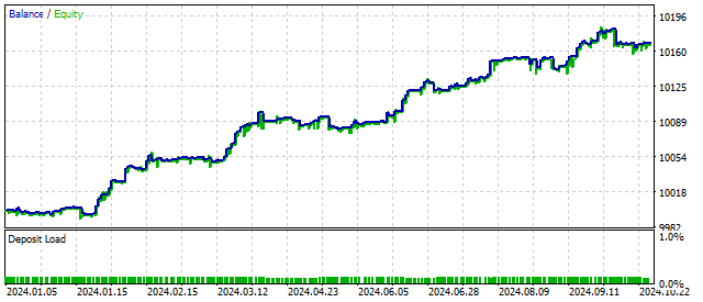
Such a model can include a wide variety of combinations of cycles and their behavior. We have seen earlier that making the model more complex improves trading results. In this case, the balance change may be as follows:

Increasing the order of the leading difference makes the model more flexible. The generalized oscillator will only react to certain price combinations. In other words, it looks for certain patterns. At the same time, you need to remember that the higher the order of the oscillator, the less often its patterns will occur.

Another feature of this algorithm is that the ratios can vary within very wide limits. Even assessing these limits can be difficult. On the other hand, the selection of ratios allows you to configure the algorithm in such a way that it will respond to non-cyclical patterns in price behavior.

Non-linear oscillators

Linear models are simple and intuitive. But price behavior on the market can also be non-linear. For example, a sharp change in price is easier to describe using non-linear models. The main advantage of non-linear models is that they can describe very complex time series behavior. When you hear the words "chaos and "stochasticity", then most probably you are dealing with non-linear models.

One of the simplest models is the signature oscillator. Its equation is in many ways similar to the harmonic oscillator. The sign function is used as a non-linear function. The trading algorithm equation looks like this:

where 'sign' is the sign function.

Thanks to this feature, the oscillator can operate in 5 different modes. Switching modes depends on the price movement. The non-linearity of the oscillator gives us hope that trading with its help will be more flexible and stable. The balance change using this algorithm might look like this:

Now, let's consider an oscillator with quadratic non-linearity. Its equation is very simple:

In order to apply this equation in practice, we need to refine it a little.

First of all, we need an average level around which the price fluctuates. Let me remind you that instead of real prices we can use their smoothed value (SMA). Then the average level will be equal to the average value of the moving averages.

Calculating the average of averages may seem a bit scary at first. In 1910, Andrey Markov published his work "Calculating Finite Differences". In this work, he showed that taking an average of a large number of SMAs is equivalent to applying an LWMA to all values of the time series. Once again, finite differences have simplified the calculations.

The equation for the quadratic oscillator trading algorithm will be as follows:

Quadratic non-linearity allows switching the oscillator operating modes more smoothly, but with a larger amplitude. This can improve trading results.

Another example of quadratic non-linearity is van der Pol oscillator. This oscillator was one of the first examples of simulating deterministic chaos. Due to its properties, the Van der Pol equation has found application not only in oscillation theory, but also in other areas - physics, biology, etc.

The van der Pol oscillator itself is a modification of the oscillator with quadratic non-linearity, and the equation for its trading algorithm looks like this:

At first glance, this oscillator should be unstable. In fact, its parameters can change over a fairly wide range without affecting trading results.

In 1918, Georg Duffing investigated the equation of an oscillator with cubic non-linearity. This oscillator can also simulate chaotic price behavior. But it has one more feature: depending on external conditions and its parameters, this oscillator can be in two stable states.

The equation of the Duffing Oscillator trading algorithm is the sum of a 3rd degree harmonic oscillator and cubic binomial:

The performance of this oscillator is comparable to other non-linear models.

In general, a lot of non-linear models can be created. Any non-linear function can become a chaos generator. The non-linearity of the three previous oscillators was based on some physical principles and ideas. Econophysics is a useful direction, but it is not at all necessary to follow it at all times.

For example, I will add non-linearity to the trading algorithm based on the logarithmic function:

You may ask: where did these logarithms come from, and on what grounds did I add them? My answer will be very simple - I wanted it that way.

But if I have time to think about the answer, it will be a little different. What is the difference between consecutive prices? Let's say 100 points. And what about the difference between the logarithms of these prices? Will there be anything there besides zeros? Here is my new answer: on the left we have a regular oscillator, and on the right we have a filter that can influence the opening of positions. The filter will only show itself when the price moves strongly. We check its work.

The result is similar to the operation of an oscillator with quadratic non-linearity. The filter is working. But it is important to remember that all ideas should first be tested in the tester before applying them in practice.

External forces

So far we have been looking at autonomous oscillators. Imagine a pendulum. It swings evenly from side to side. Its cycles repeat over and over again. Why this pendulum swings, why it swings in this particular way - these are questions we cannot answer. This is an example of a free-running oscillator.

Now, push that pendulum. First one way, then the other. The pendulum cycles began to change - its instantaneous frequency and amplitude changed. Under the influence of external forces, the pendulum ceased to be autonomous.

Let's try to apply the same approach to the harmonic oscillator. Its equation will change and look like this:

where F[n] is an external force. What kind of force is this, how does it act, where is it directed - I know nothing about it. I just assume that it exists. And now the question arises: is such a complication of the model justified? Let's answer it.

I obtained this result by assuming that this external force is related to price values as follows:

I made this assumption for only one reason - I talked about finite differences throughout the article, and in this case I also used the ratios of the 2nd difference. You are free to make your own assumptions. For example, external force may be related to the difference between closing and opening prices, tick volumes, etc. You can also add an element of non-linearity:

After all, this unknown force may depend on several components. Summarize as much as you can as long as possible. Any assumption you make can have a positive impact on your trading results.

Conclusion

As you can see, using cyclical patterns in trading is quite justified. The main advantage of such models is that they have hundreds of combinations of parameters that give a stable result over a long period of time. The trader needs to select several dozen options that do not correlate with each other.

In this article, I have only touched upon a few of the most popular oscillators. There are still quite a few solutions that can be used to build cyclic models (among other things).

I tested the EA under the following conditions: EURUSD, H1, 2024.01.01 - 2024.10.30

The following programs were used in writing this article:

Name	Type	Description
Harmonic Oscillator	EA	iPeriod - moving average period Type - moving average type R - oscillator ratio, permissible value: 1 ... 399
Damped Harmonic Oscillator	EA	S - dumping ratio, permissible value: -1000 ... +1000
scr Elliott wave	script	A1, A2 - amplitudes of sinusoids N1, N2 - periods of sinusoids Width - line width Pause - delay in displaying the result Screenshot - if 'true', then the image is created and saved in the Files folder
Elliott wave	EA	R, S - oscillator ratios, acceptable value: 0 ... 1000
Generalized Harmonic Oscillator	EA	permissible value of ratios: -1000 ... +1000
Sign Oscillator	EA
Quadratic Oscillator	EA
Van der Pol Oscillator	EA
Duffing Oscillator	EA
Log Oscillator	EA
Non-Autonomous Oscillator	EA