Rebuy algorithm: Math model for increasing efficiency

Contents

• Introduction
• Methods for refining trading characteristics based on the averaging algorithm
• "Help me get out of the drawdown"
• General thoughts about the averaging algorithm
• Subtleties of a more accurate assessment of rebuy systems
• In-depth and universal understanding of profitability
• Universal assessment
• Examples of clarifying methods
• Increasing the efficiency of systems with diversification
• Useful limits
• Useful features in terms of using parallel tools
• Normal distribution of a random variable
• Profit curve beauty in the framework of the random values distribution law
• Conclusion

Introduction

This trading method is actively used in a wide variety of Expert Advisors. Moreover, it has many varieties and hybrids. In addition, judging by the number of references to such systems, it is obvious that this topic is very popular not only on this site, but also on any other web resources. All method varieties have a common concept involving trading against the market movement. In other words, the EA uses rebuys to be able to buy as low as possible and sell as high as possible.

This is a classic trading scheme that is as old as the world. In one of the previous articles, I partially touched on this topic, while highlighting possible ways to hybridize such methods. In this article, we will have a closer look at the concept delving deeper than forum users do. However, the article will be more general and much broader as the rebuy algorithm is very suitable for highlighting some very interesting and useful features.

Methods for refining trading characteristics based on the averaging algorithm

"Help me get out of the drawdown" (from the authors of "my EA makes good money, but sometimes blows up the entire account")

This is a common issue of many algorithmic and manual traders. At the time of writing this article, I had a conversation with such a person, but he did not grasp my point of view in its entirety. Sadly, it seems to me that he has practically no chance of ever understanding the whole comedy of such a situation. After all, if I could once ask a similar question to my older and more experienced self, I would also most likely be unable to understand the answer. I even know how true answers to myself would make me feel. I would think that I am being humiliated or dissuaded from further engaging in algorithmic trading.

In reality, everything is much simpler. I just had the patience to walk a certain path and gain some wisdom, if you can call it that. This is not an idealization and self-praise, but rather a necessary minimum. It is a pity that this path took years instead of weeks and months.

Here we have a whole world of dreams and self-deception, and to be honest, I am already starting to get tired of the simplicity of some people. Please stop doing nonsense and thinking that you are the kings of the market. Instead, contact an experienced person and ask them to choose an EA for your budget. Trust me, you will save a lot of time and money that way, not to mention your sanity. One of those persons has written this article. The proofs are provided below.

General thoughts about the averaging algorithm

If we have a look at the rebuy algorithm, or "averaging", it first may seem that this system has no risk of loss. There was a time when I did not yet know anything about such tricks and was surprised at the huge mathematical expectations that beat any spreads. Now it is clear that this is only an illusion, nevertheless, there is a rational grain in this approach, but more on that later. To begin with, in order to be able to objectively evaluate such systems, we need to know some indirect parameters that can tell us a little more than a simple image of growing profits.

The most relevant parameters in the strategy tester report can even help to understand that the system is obviously losing, despite the fact that the balance curve looks great. As you might have already understood, it is really all about the profitability curve. In fact, all the important indicators of the trading system are secondary to the first and most basic mathematical characteristics, which, of course, are the mathematical expectation and its primary characteristics. But it is worth noting that the mathematical expectation is such a flexible value that you can always fall into the trap of wishful thinking.

In fact, in order to correctly use such a concept as mathematical expectation, one must first of all understand that this is the terminology of probability theory, and any calculation of this quantity should be carried out according to the rules of probability theory, namely:

• Calculations are the more accurate, the larger the analyzed sample, ideally the exact value is calculated from an infinite sample.
• If we break infinity into several parts, we get several infinities

Someone might think how to calculate the exact mathematical expectation of a particular strategy, if we have only a limited sample of real quotes at our disposal. And someone will think, why do we need these infinities at all. The thing is that all estimates of certain averaged values, such as mathematical expectation, have weight only in the area where these calculations were made, but have nothing to do with another area. Any mathematical characteristic has weight only where it is calculated. Nevertheless, some techniques can be distinguished to refine the characteristics of the profitability of a particular strategy, which will make it possible to obtain the values that are closest to the true values of the required parameters.

This is directly related to our task. After realizing that we cannot see into the future of an infinity-long strategy, which in itself already sounds like complete nonsense. Nevertheless, this is a mathematical fact and a necessary and sufficient condition for calculating the true mathematical characteristics. We come to the idea of how to make the number calculated on a limited sample closer to the number that could be calculated on an infinite sample. Those who are familiar with mathematics know that there are two mathematical concepts which can be applied to calculate infinite sums:

• Integral
• Sum of infinite series

I think it is clear to everyone that in order to calculate the integral, as well as the sum of the series, it is necessary to obtain either all points of the function, the integral of which needs to be calculated, within the considered area of integration, or all elements of the sequence of numbers within the series under consideration. There is still the most perfect option - getting the appropriate mathematical expressions for the function that we are going to integrate, and the expression for generating the elements of the series. In many cases, if we have the appropriate mathematical expressions, we can get the exact equations for the finished integral or the sum of the series, but in the case of real trading, we will not be able to apply differential calculus, and in general this will not help us much, but it is important to understand.

The conclusion from all this is that for the direct evaluation of any system we have only a limited sample and certain parameters that we get in the strategy tester. In fact, their significance is greatly exaggerated. The question arises as to whether it is possible to judge the profitability of a particular strategy using the the strategy tester parameters, whether these parameters are sufficient for an unambiguous answer and most importantly, how to use these parameters correctly and whether we really use them correctly.

Additionally, we need to understand that for each strategy, any parameter, by which we can correctly assess the real profitability and security of the strategy can be completely different. This is directly related to the evaluation of the profit curve. To understand this, let's first draw an approximate general view of the trading curve that we get when using the rebuy algorithm:

Fig. 1

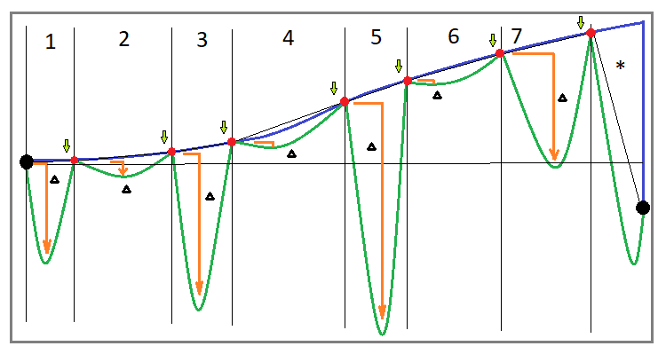
Let's start with the implementation of a rebuy for one instrument. If you correctly implement this algorithm, then your trading will in any case consist of cycles. Ideally, all cycles should be positive. If some cycles close in the negative zone, then either you are implementing this algorithm incorrectly, or it is no longer a pure algorithm and there are already modifications in it. But we will consider the classic rebuy. Let's define some characteristic parameters of the trading curve to denote a classic rebuy:

• The balance curve must be growing and consist of N cycles
• All cycles have a positive profit
• When trading breaks, we are likely to find ourselves in the last incomplete cycle
• Incomplete cycle has negative profitability
• Cycles have characteristic drawdowns in terms of funds.

It seems that the general appearance of the curve should make it clear at first glance that such a system is profitable, but not everything is so simple. If you look at the last unfinished trading cycle, which I specifically closed below the starting point, you will see that in some cases you will be lucky and you will wait for the successful completion of the cycle, while in some cases you may either not wait till the end and face a big loss or blow up your deposit entirely. Why is this happening? The thing is that the image may give a false impression that the amount of drawdown by funds is limited in its absolute value and, as a consequence, the time spent in this drawdown should also be limited.

In reality, the longer the testing area, the longer the average drawdown area. There is absolutely no limit here. The limit exists only in the form of your deposit and the quality of your money management. However, a competent approach to setting up your system based on this principle, can only lead to an increase in the lifespan of your deposit before it is eventually blown up or,at best, makes a very little profit.

When it comes to testing systems based on the rebuy (averaging) algorithm, in order to correctly assess its survivability, reliability and real profitability, one should adhere to a special testing structure. The whole point is thatthe value of a single test in this approach is minimized for one simple reason, that when testing any "normal" strategy, your profit for the entire test in the strategy tester is very close to the "normally" distributed value. This means that when testing any average strategy without holding a position for a long time, you will get an approximately equal number of profitable and unprofitable testing areas, which will very quickly let you know that the strategy is unstable, or that the strategy has a correct understanding of the market and works on the entire history.

When we are dealing with a rebuy strategy, this distribution can be strongly deformed, because for the correct testing of this system you need to set the maximum possible deposit. In addition, the test result is highly dependent on the length of the test section. Indeed, in this approach, all trading is based on trading cycles, and each unique setting of this system can have both a completely different parameter of the average drawdown and the parameter of the average duration of the drawdown associated with it. Depending on these indicators, too short test sections can show either too high or too low test result. As a rule, few such tests are carried out, and this can in most cases be the cause of excessive confidence in the operation of these systems.

Subtleties of a more accurate assessment of rebuy systems

Now let's learn how to correctly evaluate the performance of systems using the rebuy algorithm, while applying the known parameters of trading systems. First of all, with such an assessment, I would advise using one single characteristic - recovery factor. Let's figure out how to count it:

• Recovery Factor = Total Profit / Max Equity Drawdown
• Total Profit - total profit per trading area
  
• Max Equity Drawdown - maximum drawdown of equity relative to the previous joint point for balance and equity (balance peak)
  

As we can see, this is the final profit divided by the maximum drawdown of the funds. The mathematical meaning of this indicator in the classical sense is that, according to the idea, it should show the system's ability to restore its drawdown by equity. The boundary condition for the profitability of a trading system when using such a characteristic is the following fact:

• Recovery Factor > 1
  

If translated into understandable human language, it will mean that in order to make a profit, we can risk no more than the same amount of the deposit. This parameter in many cases provides an accurate assessment of trading quality for a particular system. Use it, but be very careful, because this is a rather controversial value regarding its mathematical significance.

Nevertheless, I will have to reveal you all its disadvantages, so that you understand that this parameter is also very arbitrary and the level of its mathematical significance is also very low. Of course, you might say if you criticize something, then offer an alternative. I will certainly do that, but only after we analyze this parameter. This parameter is tied to the maximum drawdown, which, in turn, can be tied to any point on the trading curve, which means that if we recalculate this drawdown relative to the starting balance and substitute it for the maximum drawdown, we almost always get an overestimated recovery factor. Let's formalize it all properly:

• Recovery Factor Variation 1 =  Total Profit / Max Equity Drawdown From Start
• Max Equity Drawdown From Start - maximum drawdown from the starting balance (not from the previous maximum)
  

Of course, this is not a classical recovery factor, but in its essence it actually determines profitability much more correctly relative to the generally accepted boundary condition. Let's first visually depict both options for calculating this indicator - the classic one and mine: 

Fig. 2

It can be seen that in the first case, this parameter will take higher values, which, of course, is what we want. But from the point of view of profitability assessment, two approaches can be followed. The classic parameter is more adapted to the approach, in which it is better to take the duration of the testing section as long as possible. In this case, a higher value of Max Equity Drawdown compensates for the fact that this drawdown does not start from the very beginning of the trading curve, and thus this parameter in most cases is close to the true estimate. My parameter is more efficient when evaluating multiple backtests.

In other words, this parameter is more accurate the more tests of your strategy you have done. The tests of your strategy should be in as many different areas as possible. This means that the start and end points should be chosen with maximum variability. For a correct assessment, it is necessary to select "N" of the most different areas and test them, and then calculate the arithmetic average of this indicator for all testing areas. This rule will allow us to refine both versions of the recovery factor, both mine and the classic one, with the only amendment that fewer independent backtests will need to be performed to refine the classic one.

Nevertheless, saying that such clarifying manipulations are few for clarifying these parameters would be an understatement. I have demonstrated my own version of the recovery factor in order to show that anyone can come up with their own similar parameter, and it can even be added as one of the calculated characteristics for backtesting in MetaTrader. But any of these parameters does not have any mathematical proof, and moreover, any of these parameters has its own errors and limits of applicability. All this means that at the moment there is no exact mathematical indicator for an absolutely accurate assessment of one or another algorithm using rebuy. However, my parameter will tend to the absolute accuracy with an increase in the number of various tests. I will provide more details in the next section.

In-depth and universal understanding of profitability

Universal assessment

I believe, everyone knows that such parameters as the mathematical expectation of profit and the profit factor exist in any strategy tester report or in the characteristics of a trading signal, but I think no one told you that these characteristics can also be used to calculate profitability of such trading systems where there is not enough analysis of deals. So, you can use these parameters by replacing the "position" unit with "test on the segment". When calculating this indicator, you will need to make many independent tests with no consideration to any structure inside. This approach will help you assess the real prospects of the trading system using only the two most popular parameters. In addition, it can instill in you an extremely useful habit - multiple tests. In order to use this approach, you only need to know the following equation:

where:

• M - expected payoff value
• Wp - desired profit
• Investments - how much you are willing to invest to achieve the required profit
• P - probability that we will have enough investment until the profit is achieved
• (1-P) - probability that we will not have enough investment until the profit is achieved (deposit loss)

Below is a similar equation for the profit factor:

All you need to know is that with random trading and the absence of obstacles such as spread, commission and swap, as well as slippage, these variables will always take the following values for any trading system:

M=0

Pf=1

These characteristics can change in your direction only if there is a predictive moment. Therefore, the probability that we will make a profit without losing the deposit will take the following value:

If you substitute this expression for probability in our equations, then you will get the identities that I provided. If we consider spread, commission and swap, then we get the following:

The spread, commission and swap reduce the final probability, which ultimately leads to the identities losing their validity. The following inequalities appear instead:

• M < 0
• Pf < 1

This will be the case with absolutely any trading system, and the rebuy algorithm here is absolutely no better than any other system. When testing or operating such a system, it is able tostrongly deform the distribution function of the random value of the signal or backtest final profit, but typically this scenario occurs most frequently during short-term testing or operation.

This is because the probability of running into a large drawdown is much less if you test on a short section. But once you start doing these tests over longer segments, you will usually see things you have not seen before. But I am sure most will be able to reassure themselves that this is just an accident, and you just need to somehow bypass these dangerous areas. The same will generally be the case with multiple testing on short segments.

There is only one way to overcome the unprofitability of any system. Let's add an additional component to the probability calculation equation:

As we can see, the new component "dP(Prediction)" has appeared in the equation. It has a plus sign, which I did on purpose to show that only this component is able to compensate for the effect of spreads, commissions and swaps. This means that we first of all need sufficient prediction quality to overcome the negative effects and reach profit:

We can get our desired inequalities only if we provide this particular inequality:

• M > 0
• Pf > 1

As you can see, these expressions are very easy to understand, and I am sure that no one will doubt their correctness. The next subsection will be easier to understand using these equations. Indeed, I advise you to remember them, or at least remember their logic, so that you can always restore them in memory if necessary. The main thing here is their understanding. In general, one of these equations is sufficient, but I felt that it would be better to show two for an example. As for other parameters, I believe, they are redundant within the framework of this section.

Examples of clarifying methods

In this subsection, I want to offer you some additional refinement manipulations that will allow you to get a more correct value of the recovery factor. I suggest going back to "Figure 1" and looking at the numbered segments. To refine the recovery factor, it is necessary to imagine that these segments are independent tests. This way we can do without multiple testing, assuming that we have already performed these tests. We can do this because these segments are cycles that have both a start point and an end point, which is what provides equivalence to the backtest. 

Within the framework of this section, I think it is also worth supplementing the first image with its equivalent considering the fact that we are testing or trading on several instruments at once. This is how the trading curve will look like using the rebuy algorithm for parallel trading on multiple instruments:

Fig. 3

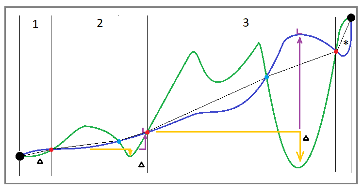
We can see that this curve differs in its structure from the curve for rebuying on one instrument. I have added intermediate blue points here, which means that before the drawdown there may be segments that have a "drawdown in reverse." The fact is that we cannot consider this a drawdown. But nevertheless, we have no right to consider these segments outside the analysis. This is why they must be part of a cycle.

I think it would be more correct to postpone each new cycle from the end of the previous one. In this case, the end of the previous cycle should be considered the recovery point of the last drawdown in equity. In the image, these cycles are separated by red dots. But in fact, this definition of the cycle is not sufficient. It is also important to determine that it is not enough just to fix the drawdown by equity, but it is important that it be lower than the start of the current cycle. Otherwise, what kind of drawdown is it?

After highlighting these cycles, you can consider them as separate independent tests and calculate the recovery factor for each of them. This can be done the following way:

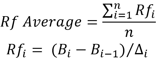
In this equation, the corresponding points on the balance curve (the final value of the balance on the section and the initial one) are used as "B", while the delta represents our drawdown. I would also like the reader to return to the last image. On it, I plotted the delta from the red start point of each cycle, and not from the blue one, as is usually the case, for the reasons I listed above. But if you need to clarify the original recovery factor, then the delta should be plotted from the blue point. In this case, the method of refining the parameters is more important than the parameters themselves. The simple arithmetic mean is taken as the averaging action.

Nevertheless, even after clarifying one or another custom or classic parameter, you should not take the fact that the value of this indicator is more than one, or even two or three, as signs of a profitable trading system.

Exactly the same equation should be applied with multiple backtests. The point is that any backtest in this case is equivalent to a cycle. We can even first calculate the averages for the cycles, and after all this, calculate the average of the average relative to the backtests. Or we can do it much easier by maximizing the duration of the test segment. This approach will save you at least from multiple tests due to the fact that the number of cycles will be at maximum, which means that the average recovery factor will be calculated as accurately as possible.

Increasing the efficiency of systems with diversification

Useful limits

After considering the possibilities to refine certain characteristics of backtests, you are undoubtedly better armed, but you still do not know the main thing. The basis lies in the answer to the question - why is it necessary to carry out all these multiple tests or splitting into cycles? The question is really complex until you put in as much effort as I put in my time. Sadly, this is necessary, but with my help, you can greatly reduce the time you need to do this.

This section will allow you to evaluate the objectivity of a particular parameter. I will try to explain both theoretically and using the equations. Let's start with the general equation:

Let's consider a similar equation with some slight changes:

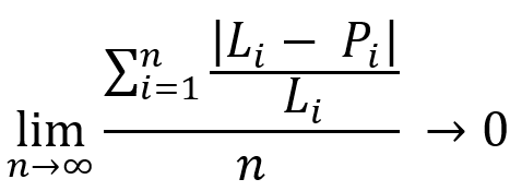
The essence of these equations is the same. These equations demonstrate thatin any profitable trading system, when the duration of the testing section tends to infinity, we will get a complete merger of the balance and current profit lines, with a certain line representing our average profit. In most cases, the nature of this line is determined by the strategy we have chosen. Let's look at the following image for a deeper understanding:

Fig. 4

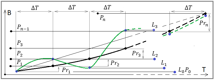
If you carefully look at this image, you will see on it all the quantities that are present in our equations. It reveals the geometric meaning of our mathematical limits. The only thing missing in our equations is the dT time interval. With this interval, we discretize our balance steps and give rise to all the points of our number series for the balance and profit of these intervals, and also calculate the values of our midline at the same points. These equations are the mathematical equivalent of the following statement:

• The more we combine multiple tests or trading curves together, the more they look like a smooth rising line (only if the system is really profitable)

In other words, any profitable trading system looks more beautiful in the graphical part of the strategy tester or signal, the longer the testing area we choose. Some might say that no system can achieve such indicators, nevertheless, there are plenty of examples in the Market, so it would be silly to deny this. It all depends on the universality of the algorithm and how well you understand the market physics. If you know the math that is always inherent in the market you are trading, then in fact you get an infinitely growing profit curve, and you do not need to wait for an entire infinity to confirm the effectiveness of the system. Of course, it is clear that this is an extremely difficult task, but nevertheless, within the framework of many algorithms, this task is achievable.

Let's finish this theoretical introduction by learning how to use the received techniques correctly. You might ask, how to use these techniques with infinite sums, when we have only limited samples and, accordingly, also inevitable incomplete sums.

1. The answer lies is in dividing the entire history into segments
2. Select several segments with a constantly growing length for the duration of testing up to a segment in the entire history
3. Choose a testing methodology
4. Test
5. Look for an improvement in recovery factor and/or relative drawdown

The essence of this tricky test scheme is to reveal indirect signs that our limits really tend to infinity and zero, respectively. To increase the efficiency of our testing scheme, we must understand that the longest test section should at least look more beautiful than the shortest one, and ideally each subsequent section should be both larger and look more beautiful. I use the concept of "more beautiful" only to make it clear to everyone that this is actually equivalent to our limits.

However, our limits are only good during theoretical considerations or preparations (whatever you like). In this regard, the question arises - how to discover these facts without resorting to "eyeball analysis"? We need to somehow adapt our limits to the parameters that we have in the strategy tester report. In other words, we need alternative limits for some strategy tester report or signal parameters so that our testing structure can be used. Let me show you the necessary and sufficient set of alternative limits:

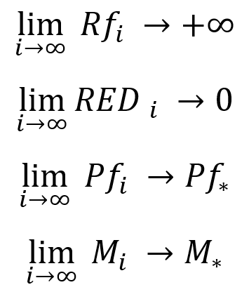
What we should understand here:

1. During an infinite test, the recovery factor of any profitable strategy tends to infinity
2. During an infinite test, relative drawdown by equity (of any profitable strategy) tends to zero
3. During an infinite test, the profit factor of deals of any profitable strategy tends to its mean value and has a finite real limit.
4. During an infinite test, the mathematical expectation of any profitable strategy without auto lot enabled (with a fixed lot) tends to its average value and has a finite real limit

All this has to do with infinite tests, however it is useful to understand the mathematical meaning of these limits before proceeding to adapt them to a finite sample. The adaptation of these expressions to our methodology should begin with the fact that we should select several segments of testing, each of which should be significantly larger than the previous one, preferably at least twice. This is necessary in order to be able to notice the difference in readings between shorter and longer tests. If we number our tests in such a way that as the index increases, its length grows in time, then we get the following adaptation for the case of finite samples:

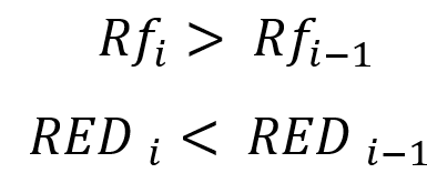
In other words, an increase in the recovery factor and a decrease in the relative drawdown in terms of funds is indirect evidence that, most probably, the further increase of the test segment or signal lifetime makes our curve become visually more beautiful. This means that we have confirmed the fulfillment of our infinite limits. Otherwise, if the profit curve does not become straighter, we can state the fact that the result obtained is very close to random and the probability of losses in the future is extremely high.

Of course, many will say that we can simply optimize the system more often and everything will be all right. In some extremely rare cases it is possible, but this approach will require a completely different testing methodology. I do not advise anyone to resort to this approach, because in this case you do not have any math, while here you have everything in a clear-cut manner.

All these nuances should convince you that testing the rebuy algorithm all the more requires the use of this approach. In particular, we can even simplify the task and test the rebuy system immediately on the maximum length segment. We may reverse this logic. If we do not like the trading performance in the longest segment, then even better performance in the short segments will indicate that our inequalities are no longer satisfied and the system is not ready for trading at this stage.

Useful features in terms of the parallel use of multiple instruments

When testing on a limited history, the question will certainly arise - is there enough history for us to correctly use our testing methodology? The thing is that in many cases the strategy has weight, but its quality is not high enough for comfortable use. To begin with, we should at least understand whether it really has a predictive beginning and whether we can begin to engage in its modernization. In some cases, we literally do not have enough available trading history. What should we do? As many have already guessed, judging by the title of the subsection, we should use multiple instruments for this purpose. 

It would seem an obvious fact, but unfortunately, as always, there is no math anywhere. The essence of testing on multiple instruments is equivalent to the same essence for increasing the duration of testing. The only amendment is that your system must be a multi-currency one. The system may have different settings for different trading instruments, but it is desirable that all settings are similar. The similarity of the settings will represent the fact that the system uses physical principles that work on the maximum possible number of trading instruments.

With this approach and the correct implementation of such tests, the index "i" should already be understood as the number of simultaneously tested instruments on a fixed testing segment. Then the expressions will mean the following:

1. When increasing the number of traded instruments, the more instruments, the greater the recovery factor
2. When increasing the number of traded instruments, the more instruments, the smaller the relative drawdown by equity

In fact, an increase in the number of tests can, for simplicity, be interpreted as an increase in the total duration of tests, as if we consider each test for each tool to be part of a huge overall test. This abstraction will only help you understand why this approach also has the same power. But if we consider this issue more accurately and understand more deeply why a line that consists of several ones will be much more beautiful, then we should use the following concepts of probability theory:

• Random value
• Variance of a random variable
• Mathematical expectation of a random variable
• The law of normal distribution of a random variable

To fully explain why we need all this, we first need an image that will help us look at a backtest or a trading signal a little differently:

Fig. 5

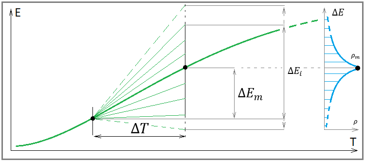
I am not drawing a balance line here, because it does not decide anything here, and we only need a profit line. The meaning of this image is thatfor each profit line, it is possible to select an infinite number of independent segments of a fixed length, in which it is possible to construct the law of distribution of a random variable of the profit line increment. The presence of a random variable means that in the future the profit increment in the selected area can have completely different values in the widest range.

It sounds complicated, but in fact all is simple. I think many people have heard about the normal distribution law. It supposedly describes almost all random processes in nature. I think, this is no more than an illusion invented to prevent you from "thinking". All jokes aside, the reasons for the popularity of the distribution law are that it is an artificially compiled and very convenient equation for describing symmetric distributions with respect to the mathematical expectation of a random variable. It will be useful to us for further mathematical transformations and experiments.

However, before starting to work with this law, we should define the main property for any distribution law of a random variable:

Any law of random variable distribution is essentially the analogue of the full group of non-joint events. The only difference is that we do not have a fixed number of these events and at any time we can select any event of interest like this:

Strictly speaking, this integral considers the probability of finding a random variable in the indicated range of a random variable, and naturally, it cannot be greater than one. No total event from a given event space can have a probability greater than one. However, this is not the most important thing. The only important thing here is that you should understand that the event in this case is determined only by a set of two numbers. These are examples for random variables of minimum dimension.

There are analogues of these equations for the "N" dimension, when an event can be determined by "N*2" numbers, and even more complex constructions (within the framework of multidimensional region integrals). These are quite complex sections of mathematics, but here they are redundant. All laws obtained here are self-sufficient for the one-dimensional variant.

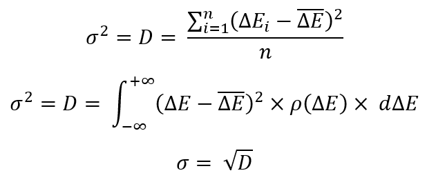
Before moving on to more complex constructions, let's recall some popular parameter characteristics of the random value distribution laws:

To define any of these equations, we need to determine the most important thing - the mathematical expectation of a random variable. In our case, it looks as follows:

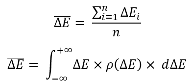
The mathematical expectation is simply the arithmetic mean. Mathematicians like to give very clever names to simple things so that no one understands anything. I have provided two equations. Their only difference is that the first one works on a finite number of random variables (limited amount of data), and in the second case, the integral over the "probability density" is used.

An integral is the equivalent of a sum, with the only difference being that it sums up an infinite number of random variables. The law of a random variable distribution, which is located under the integral and contains the entire infinity of random variables. There are some differences, but in general the essence is the same.

Now let's go back to the previous equations. These are just some manipulations with the laws of random variables distribution that are convenient for most mathematicians. As in the last example, there are two implementations - one for a finite set of random variables, the other for an infinite one (the law of a random variable distribution). It states that "D" is the average square of the difference between all random variables and the average random variable (the mathematical expectation of the random variable). This value is called "dispersion". The root of this value is called the "standard deviation".

Normal distribution of a random variable

It is these values that are generally accepted in the math of random variables. They are considered the most convenient for describing the most important characteristics of the random distribution laws. I disagree with this notion, but nevertheless I am obliged to show you how they are calculated. In the end, these quantities will be needed to understand the normal distribution law. It is unlikely that you will easily find this information, but I will tell you that the normal distribution law was invented artificially with only a few goals:

• A simple way to determine the distribution law symmetrical to the mathematical expectation
• Ability to set dispersion and standard deviation
• Ability to set mathematical expectation

All these options allow us to get a ready-made equation for the law of a random variable distribution called the normal distribution law:

There are other variations of the laws of random variables distribution. Each implementation is invented for a certain range of problems, but since the normal law is the most popular and well-known, we will use it as an example to prove and compile the mathematical equivalent of the following statements:

• The more instruments traded in parallel for a profitable system, the more beautiful and straighter our profit graph (a special case of diversification)
• The longer the selected area for testing or trading, the more beautiful and straighter our profit graph
• The more parallel traded systems with proven profitability, the straighter and more beautiful our overall profitability graph
• The combination of all of the above gives rise to ideal diversification and the most beautiful chart

Everything that has been said applies only to trading systems whose profitability has been proven mathematically and practically. Let's start by defining what "the more beautiful graph" means in mathematical terms. The "standard deviation", whose equation I have already shown above, can help us with that.

If we have a family of distribution density curves for a random variable of profit increment with the same mathematical expectation, which symbolize two segments of the same duration in time, for two practically identical graphs, then we would prefer the one with the smallest standard deviation. The perfect curve in this family could be one with zero standard deviation. This curve is achievable only if we know the future, which is impossible, nevertheless, we must understand this in order to compare curves from this family.

Profit curve beauty in the framework of the random values distribution law

This fact is understandable when we are dealing with a family of curves, where the mathematical expectations of the profit increment in the selected time period are the same, but what to do when we are dealing with completely arbitrary distribution curves? It is not clear how to compare them. In this regard, the standard deviation is no longer perfect and we need another more universal comparison value that takes into account scaling, or we must come up with some algorithm for reducing these distribution laws to a certain relative value, where all distributions will have the same mathematical expectation and, therefore, classical criteria will apply to all curves. I have developed such an algorithm. One of the tricks in it is the following transformation:

The family of these curves will look something like this:

Fig. 6

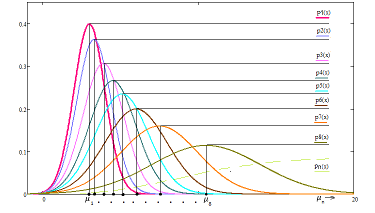
A very interesting fact is that if we subject the law of normal distribution to this transformation, then it is invariant with respect to this transformation and will look like this:

The invariance consists in the following replacements:

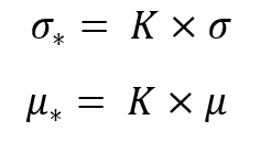
If we substitute these replacements into the previous equation, then we get the same distribution law operating with the corresponding values with asterisks:

This transformation is necessary to ensure not only the invariance of the transformation law but also the invariance of the following parameter:

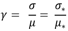
I had to invent this parameter. It is impossible to properly scale the normal distribution law, like any other law, without it. This parameter will be invariant for any other distribution law as well. As a matter of fact, the normal law is easier to perceive and understand. Its idea is that it can be used for any distributions with different mathematical expectations and its essence will be similar to the standard deviation, only without the requirement that all compared distributions must have the same mathematical expectation. It turns out, our transformation is designed to get a family of distributions where a given parameter has the same value. Seems pretty convenient, doesn't it?

This is one way to define the so-called graph beauty. The system having the smallest parameter is "the most beautiful". This is all good, but we need this parameter for a different purpose. We set the task to compare the beauty of the two systems. Imagine that we have two systems that trade independently. So, our goal is to merge these systems and understand whether there will be an effect from this merger, or rather, we hope for the following:

 

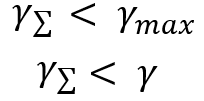
These ratios will be observed when using any distribution law. This automatically means that it makes sense to diversify if our parallel traded instruments or systems have similar profitability. We will prove this fact a bit differently. As I said, I came up with an algorithm for reducing all distributions to a relative random value. We will use it, but first we will analyze the general process of merging several lines, within the framework of the distribution law of a random variable representing the sum of two deltas. We will recurrent logic for merging in pairs. To do this, we assume that we have "n+1" curves, each of which has a defined mathematical expectation. But in order to get to the random variable symbolizing the merge, we need to understand that:

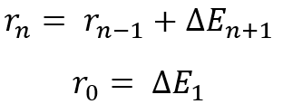
In fact, this is a recurrent expression making no mathematical sense, but it shows the logic of merging all random variables present in the list. To put it simply, we have "n+1" curves, which we must combine using "n" successive transformations. In fact, this means that we must obtain the distribution law of the total random variable at each of the steps using some kind of transformation operators.

I will not delve into lengthy explanations. Instead I will simply show these conversion operators so that you can make your own conclusions. These equations implement the merging of two profit curves within the selected time period, and calculate the probability that the total profit of the two segments of the curves "dE1 + dE2" will be lower (Pl) and higher (Pm) of the "r" selected value, respectively:

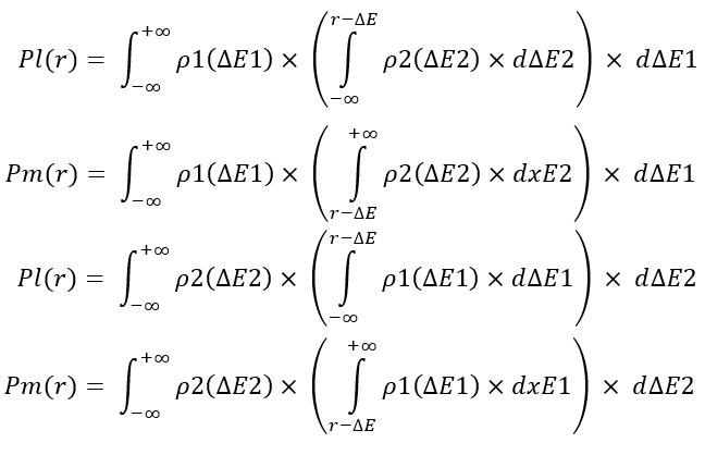
There are two options for implementing these quantities here. Both are completely similar. After calculating these values, they can be used to obtain the law of distribution of the "r" random variable, which is what is required of us to work out the entire recurrent merging chain. By definition of a random variable, we can obtain the corresponding distribution laws from these equations as follows:

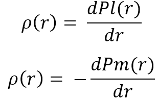
As you may have guessed, after obtaining the distribution law, we can proceed to the next step within the recurrent chain of transformations. After working through the entire chain, we get the final distribution, which we can already compare with one of the distributions that we used for the recurrent merge chain. Let's create a couple of distributions based on the laws we have got, and run one merge step as an example to demonstrate the fact that each merge is "more beautiful than the last":

Fig. 7

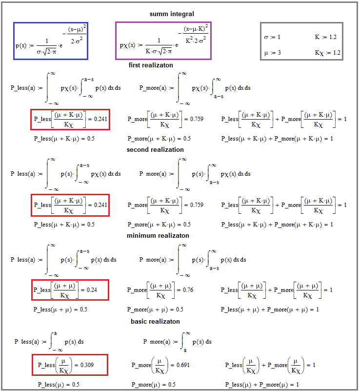
The image demonstrates the mathematical merging which applies our merging equations. The only thing not shown there is differentiation to transform integrals into laws of a random merging value distribution. We will look at the result of differentiation a little later, within the framework of a more general idea, but for now let's deal with what is in the image.

Pay attention to the red rectangles. They are the basis here. The lowest integral says that we take the integral according to the original distribution law in such a way as to calculate the probability that the random variable will take a smaller value than the mathematical expectation divided by "Kx". Above you will see similar integrals for the mergers of two slightly different distributions. In all cases, it is important to maintain this ratio (Kx) between the mathematical expectation and the chosen boundary value of the integral, which is expressed in the corresponding "Kx". 

Note that both merge options are presented there, according to the equations I gave you above. Besides, there is a merge of the base distribution with itself, as if we are merging two similar profit curves. Similar does not mean identical in the picture, but rather having identical distribution laws for the random variable of the profit curve increment in the selected time period. The proof is that we found a smaller probability of a relative deviation of the merging random variable relative to the original. This means that we have a more "beautiful" law for the increment of a random profit value in any merger. Of course, there are exceptions requiring a deeper dive into the topic, but I think this approach is enough for the article. You will most likely not find anything better anywhere, because this is a very specific material.

The alternative way to compare beauty is to transform all, both the original distribution laws and the result of the recurrent chain considered above. To achieve this, we just have to use our transformation, which allowed us to get a family of scalable distribution curves and do as follows:

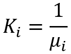
The trick of this transformation is that with this approach, all distribution laws subjected to the corresponding transformation, will have the same mathematical expectation and, accordingly, we can use only standard deviation to evaluate their "beauty" without having to invent any exotic criteria. I have shown you two methods. It is up to you to choose the one that suits you best. As you may have guessed, the distribution laws of all such relative curves will look like this:

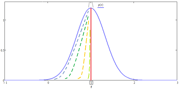
This approach is applicable to extended tests as well. By extended tests here we mean testing over a longer segment. This application is only suitable for confirming the fact thatthe longer the test, the more beautiful the graph. The only trick for this proof that you have to apply is to accept that if we increase the duration of the test, then we do it in multiples of an integer, while in multiples of this number we already consider not 1 step but "n" and apply the merge equations. This merge will be even simpler, since the recurrent merge chain will contain only a single element that is duplicated, and it will be possible to compare the result only with this element.

Conclusion

In the article, we considered not the rebuy algorithm itself, but a rather much more important topic that gives you the necessary mathematical equations and methods for a more accurate and efficient evaluation of trading systems. More importantly, you get the mathematical proof of what diversification is worth and what makes it effective, and how to increase it in a natural and healthy way, knowing that you are doing everything right.

We have also proved that the graph of any profitable system is more beautiful, the longer the trading area we use, and also, the more profitable systems trade simultaneously on one account. So far, everything is framed in the form of a theory, but in the next article we will consider the applied aspects. To put it simply, we will build a working mathematical model for price simulation and multi-currency trading simulation and confirm all of our theoretical conclusions. You most likely will not find this theory anywhere, so try to delve deeper into this math, or at least understand its essence.