MQL5 Wizard Techniques you should know (Part 76): Using Patterns of Awesome Oscillator and the Envelope Channels with Supervised Learning

Introduction

From our last article, we introduced the indicator pairing of the Awesome-Oscillator and the Envelope-Channels, and from the testing of that pair 7-8 of the 10 patterns walked forward on a 2-year test window. We usually follow up the introduction of an indicator pair with an exploration of what impact, if any, machine learning can have on the performance of these indicator signals. This article is no exception, and thus we are going to examine how the patterns 4,8,and 9 can be affected/influenced if we supplement their signals with a supervised-learning network as a filter. For our network, we are using a CNN whose kernels/channels are sized by the dot product kernel with cross-time attention.

Dot Product Kernel with Cross-Time-Attention

This kernel is a form of attention mechanism where, given two sequences, that are usually features from different time steps or layers, one would compute an attention score between every pair by using their dot product. This approach would highlight the relationships across time and how a past or future feature is pertinent to a current one. Here’s how it works; if you have the following two sequences:

X=[x1,x2,...,xT]

Y=[y1,y2,...,yS]

For each pair (xi,yj) you would calculate the dot product score as: 

Scorei,j = xi⋅yj

Alternatively, applying a soft-max over j or i to get attention weights can be done, where the weights are then used to blend/reweight the features across time. This is useful because it is parameter efficient - not requiring extra learned parameters beyond projections. It is flexible since it can handle variable-length sequences, irregular sampling and cross modal/time interactions. It is also powerful, in that it focuses on relevant moments, not just the local convolutional neighbourhoods. Its applications are in time series forecasting especially where lag is important, video analysis where frames are linked over time, speech, and any domain where temporal/time-based dependencies are not trivial.

So, why are we selecting this kernel then to guide our CNN kernel/channel sizes? Well, for the kernels, they have spatial and temporal characteristics. Firstly, attention kernels tell you which time steps are more important. This is perhaps not as poignant in small kernel instances that are very focused, however as the kernels spread out, more context is captured. CNNs are also inherently local, therefore the attention can adaptively widen/focus the effective receptive field by influencing the kernel size depending on the data sequence’s time dynamics.

For the channels, the attention kernel can spot which feature channels or dimensions are ‘most attended to’. It is a guide to pruning the channels. If attention consistently ignores certain channels, they’re dead weight and effectively reduce the overall channel size. It is also an indicator for expansion. If attention is diffused with no clear focus, then you could need a richer representation with more channels. Our approach then, much like in past articles where we have exploited CNN enhancements, is to have a dynamic design for the CNN instead of static kernel/channel sizes of one size fits all. We use attention patterns in training and inference to reconfigure CNNs - with the goal of attaining more efficient, effective models for non-stationary financial market data.

Despite our dynamic approach that is geared towards improving model adaptability and performance, there are some drawbacks that are worth mentioning. First up, we have computation overhead of O(N^2) with input data sequence length, while static CNNs are typically O(N). For long sequences, this is prohibitive. Secondly, we have an interpretability paradox. Attention scores are ‘nice’ however merging them with dynamic kernel/channel selection does make the model more complex to interpret and meaningfully infer information from, to apply to 3rd party situations.

Also, it isn’t always better as some testing has indicated that in purely local tasks such as edge detection in images classic CNNs may outperform attention-heavy models. Furthermore, the data requirements for attention kernels are significantly more than those of the classic CNNs, during training/optimization in order to learn meaningful cross-time dependencies. Finally, there is an overfitting risk. If attention guides architectural changes, you can end up chasing noise or randomness in tested data by being overly adaptive.

Possible alternatives to our approach include: dilated convolutions where the receptive field gets expanded without increasing kernel size to cover wide but sparse temporal differences; or dynamic/adaptive convolutions where kernel weights are set based on the nature of the input data or attention signals; or we could have depthwise separable convolutions where our variable is only channel size and our goal is compute-efficiency; or we could use squeeze and excitation blocks; or temporal convolutional networks. Each of these take a novel turn on our approach with some advantages and challenges, but are presented here for completeness in showing what is possible in tuning CNNs.

The Network

With that brief intro on the dot product cross-time-attention kernel, let's get forensic on the code. The body of code to this network, as a class, is presented below:

import torch
import torch.nn as nn
import torch.nn.functional as F

class DotProductAttentionConv1D(nn.Module):
    def __init__(self, input_length=100):
        super(DotProductAttentionConv1D, self).__init__()
        self.input_length = input_length

        # Deeper and wider design with attention
        self.kernel_sizes, self.channels = self._design_architecture()

        self.conv_layers = nn.ModuleList()
        self.attention_layers = nn.ModuleList()  # For cross-time attention
        in_channels = 1

        for i, (out_channels, kernel_size) in enumerate(zip(self.channels, self.kernel_sizes)):
            # Convolutional block
            conv_layer = nn.Sequential(
                nn.Conv1d(in_channels, out_channels, kernel_size=kernel_size, padding=kernel_size // 2),
                nn.BatchNorm1d(out_channels),
                nn.ReLU(),
                nn.Dropout(0.2))
            self.conv_layers.append(conv_layer)
            
            # Attention block (cross-time attention)
            if i % 2 == 0:  # Apply attention to every other layer
                attn_layer = nn.MultiheadAttention(embed_dim=out_channels, num_heads=4)
                self.attention_layers.append(attn_layer)
            else:
                self.attention_layers.append(None)
            
            in_channels = out_channels

        # Fully connected head (same as original)
        self.head = nn.Sequential(
            nn.AdaptiveAvgPool1d(1),
            nn.Flatten(),
            nn.Linear(in_channels, 128),
            nn.ReLU(),
            nn.Dropout(0.2),
            nn.Linear(128, 64),
            nn.ReLU(),
            nn.Linear(64, 1),
            nn.Sigmoid()
        )

    def _dot_product_kernel(self, x):
        """Dot product similarity kernel with positional encoding"""
        # x shape: (B, C, L)
        x = x.permute(0, 2, 1)  # (B, L, C)
        # Compute dot product attention
        attention_scores = torch.bmm(x, x.transpose(1, 2))  # (B, L, L)
        attention_weights = F.softmax(attention_scores / (x.size(-1) ** 0.5), dim=-1)
        return torch.bmm(attention_weights, x).permute(0, 2, 1)  # (B, C, L)

    def _design_architecture(self):
        # Simulate attention response pattern
        num_layers = 10
        kernel_sizes = [3 + (i % 4) * 2 for i in range(num_layers)]  # cyclic 3, 5, 7, 9
        channels = [32 * (i + 1) for i in range(num_layers)]  # 32, 64, ..., 320
        
        return kernel_sizes, channels

    def forward(self, x):
        x = x.unsqueeze(1)  # (B, 1, L)
        
        for conv_layer, attn_layer in zip(self.conv_layers, self.attention_layers):
            x = conv_layer(x)
            
            if attn_layer is not None:
                # Reshape for attention (MultiheadAttention expects seq_len first)
                attn_input = x.permute(2, 0, 1)  # (L, B, C)
                attn_output, _ = attn_layer(attn_input, attn_input, attn_input)
                x = attn_output.permute(1, 2, 0)  # (B, C, L)
                
                # Also apply dot product kernel
                x = self._dot_product_kernel(x)
        
        return self.head(x)

Firstly, our class inherits from the nn.Module, a standard for networks using PyTorch. The parameter input-length sets the expected sequence length, however on adjustments the class can still take in input sequences of variable length. The super directive makes sure that the base class is initialized, a very important step for ‘all the magic’ to work in PyTorch, so certainly not worth skipping. With this, we move on to the architecture or kernel and channel sizing.

As introduced above, we are using a dynamic approach. In the place of hard coding, our model picks/sets kernel and channel sizes algorithmically - allowing adaptation to the attention patterns in the input data being processed at each forward pass. As a guide note, it could be prudent to link attention statistics from prior runs or meta-learning to the actual kernel/channel choices for every layer.

Once we’ve run the design-architecture function, we then get into layer construction. Here, the Module-List function lets you build a variable depth network. This step is very important when stacking layers dynamically. We then get to the layer-stacking for-loop. At this stage, for each convolutional layer, the kernel size is allotted separately. This allows for wide or narrow filters, as the case may be. The attention kernel can later inform what is optimal. Our padding which is the kernel size floor-divided by 2 provides the same padding with output length being equal to input length for most kernels. This is vital in time series, where one needs to align the time steps. Finally, batch-normalization, ReLU activation, and Drop-out, the classic Deep-learning recipe, helps stabilize training, speed up convergence and regularize the model.

Still within the for-loop, besides the convolution block of code that we mention above, we also have an ‘attention block’ of code. Here we alternately append multi-head attention layers, the core of the transformer that captures all dependencies. We perform this appending alternately and not for every layer slot, primarily to save on compute resources. This lets the model switch between a local CNN and global reasoning. Lastly, our in-channels parameter gets assigned the out-channels value. This is because each feature map channel becomes an embedding dimension - unifying the CNN and attention representations.

We then get to the final portion of our class initialisation function, where we define the fully connected head. In here we use adaptive pooling to reduce the time dimension to 1 regardless of input length since the output size is fixed, then we flatten to prepare for fully connected layers. These are dense layers that are a stack of nonlinear transforms that terminate in a single sigmoid output. This can be inferred as a binary prediction or normalized score, but it is ultimately our price trend forecast, with sub 0.5 values being bearish while those more than 0.5 being bullish. The dropout prevents overfitting at the dense layer stage.

Having looked at this network’s class initialisation, what follows is the dot product kernel function. In computing the kernel, the first thing we do, switch the input to B-L-C for easier dot products across the input data vector sequence. We then perform a batch matrix multiplication or bmm, where we efficiently compute all the pairwise dot products for each batch. GPUs can make this process even faster. We then perform a soft-max scaling, a standard for the attention kernel where the temperature is the square root of the input vector size or the embedded dimension.

We then do the final batch matrix multiplication, where we blend features from different points in time as weighted by attention. Not only that, but we then re-permute the multiplication output in order to restore it to the shape of the input vector and also prepare it for downstream use. This function is what gives the network cross time awareness which is beyond what regular convolution alone can achieve, and we call it in the network’s forward pass function.

Our next special function within the network class is the architecture design helper. We have had similar functions when customizing the CNN in past articles, and what we are doing in this situation is cycling through a range of kernel sizes in order to simulate an ‘attention-informed’ variation. We also steadily increase the channels - a classic  deep learning approach where we seek to learn more abstract and higher dimensional representations in later layers.

Our final function to the network class is, as is usually the case, the forward pass function. The first thing we do in here is pre-process the input vector by adding the extra middle dimension, or channel, that is a requirement for 1D convolutions. With this done, for each layer we then start by doing a convolution where we extract local features from the input. We then process the conditional attention, which is a check IF there is an attention layer. Recall in the initialisation function of this class we assigned these attention layers alternately and not at each slot.

If we have an attention layer, we reshape it since PyTorch’s multi-head expects a particular format (channel, batch, length) and yet we have (batch, channel, length). Once we have the attention output, we perform the dot product kernel by calling the function we defined just above. As a side note, we are using both the transformer and the dot product in a forward pass, yet only one could be used as an alternative approach. This switching can be done with the goal of establishing which algorithm ‘carries’ the accuracy of the model. The final output then gets fed into the head for classification/ regression.

Summary of Code by Section

Section	What it Does	Why it Matters
__init__ + super	Base class setup	Essential for PyTorch functionality
self.kernel_sizes, channels	Dynamic CNN design	Tailored, adaptive feature extraction
ModuleList layers	Modular, extensible architecture	Scalability, experimentation
Convolution blocks	Local feature extraction	Traditional CNN strengths, batch normalization, etc.
MultiheadAttention blocks	Global cross-time dependencies	Captures long-range dependencies
_dot_product_kernel	Explicit attention computation	Redundant/interlinked signal for cross-time links
Fully connected head	Aggregation, output	Flexible for task (classification, regression, etc.)
forward logic	Data flow through network	Ensures correct application of each operation
_design_architecture	How kernels/channels are chosen	Can be made data- or attention-driven

Awesome Oscillator Function

The indicator functions used in MQL5 do not get imported when we use the MetaTrader 5 module in Python. We therefore always need to use existing libraries or code our own. The latter option is what we have been doing, and so we’ll stick to it and implement our awesome oscillator function in Python as follows:

def Awesome_Oscillator(df: pd.DataFrame, short_period: int = 5, long_period: int = 34) -> pd.DataFrame:
    """
    Calculate the Bill Williams Awesome Oscillator (AO) and append it to the input DataFrame.
    
    AO = SMA(Median Price, short_period) - SMA(Median Price, long_period)

    Args:
        df (pd.DataFrame): DataFrame with 'high' and 'low' columns.
        short_period (int): Short period for SMA (default 5).
        long_period (int): Long period for SMA (default 34).

    Returns:
        pd.DataFrame: Input DataFrame with 'AO' column added.
    """
    required_cols = {'high', 'low'}
    if not required_cols.issubset(df.columns):
        raise ValueError("DataFrame must contain 'high' and 'low' columns")
    if not all(p > 0 for p in [short_period, long_period]):
        raise ValueError("Period values must be positive integers")

    result_df = df.copy()
    median_price = (result_df['high'] + result_df['low']) / 2
    short_sma = median_price.rolling(window=short_period).mean()
    long_sma = median_price.rolling(window=long_period).mean()
    result_df['AO'] = short_sma - long_sma

    return result_df

Our imported modules for this function include pandas for table-like/time-series manipulation - it is good at handling data frames as well as rolling window tricks. We also import NumPy, the backbone of fast maths that is used a lot under the hood, even though we do not explicitly call it here. Our function signature, the line of text after ‘def’,  is a clean one that gives hints on the types of input data required to call the function. This clarity is combined with IDE auto-completion, since default values for averaging periods are predefined. These are in line with Bill Williams’ classic settings.

Past the signature, we start off by validating the function's data input, starting with what is required. The data frame. The columns of ‘high’ and ‘low’ need to be present. This is a sanity check that prevents cryptic bugs later if columns are missing. In addition, we check to ensure that inputted periods are valid unsigned integers. By employing user-friendly error messages we force early failure which can help with meaningful diagnostics. This defensive stance in checking input data is very important in averting NaN values. Never trust outside data.

Next, we make a copy of the input data frame to ensure the original data remains in its pristine state. This is ‘non-destructive’, and it is essential for pipelines where indicator functions are layered. We then compute the median price from the copied data frame. This is a core input to the AO, and it reflects the average traded price for the bar - not just the close price, and is meant to avert the open-price/close-price whipsaw. We then work out the short and long smoothed moving averages. The use of rolling().mean() creates a moving average that is a smooth trend signal. The short vs long comparison is at the heart of oscillator logic. It measures momentum as the distance between fast and slow trends.

Finally, we append our copied data frame with a new column, ‘AO’. This is the actual AO value. When positive short term momentum is higher than the long-term and this is a bullish vibe. When negative short term momentum is lower, which is bearish of a sign of a fading rally. As highlighted in the last article, AO is zero line driven, so crossovers are significant.

Envelopes Channel Function

We implement the envelopes in Python as follows:

def Envelope_Channels(df: pd.DataFrame, period: int = 20, deviation: float = 0.025) -> pd.DataFrame:
    """
    Calculate Envelope Channels (Upper & Lower Bands) and append to the input DataFrame.

    Envelope Channels = SMA(close, period) * (1 ± deviation)

    Args:
        df (pd.DataFrame): DataFrame with 'close' column.
        period (int): Period for SMA calculation (default 20).
        deviation (float): Deviation as a decimal (e.g., 0.025 for 2.5%, default 0.025).

    Returns:
        pd.DataFrame: Input DataFrame with 'Envelope_Upper' and 'Envelope_Lower' columns added.
    """
    required_cols = {'close'}
    if not required_cols.issubset(df.columns):
        raise ValueError("DataFrame must contain 'close' column")
    if period <= 0 or deviation < 0:
        raise ValueError("Period must be positive and deviation non-negative")

    result_df = df.copy()
    sma = result_df['close'].rolling(window=period).mean()
    result_df['Envelope_Upper'] = sma * (1 + deviation)
    result_df['Envelope_Lower'] = sma * (1 - deviation)
    result_df['Envelope_Mid'] = 0.5 * (result_df['Envelope_Upper'] + result_df['Envelope_Lower'])

    return result_df

As with the AO, the signature is type-hinted and ‘sane’ default values are used for the inputs of period and deviation. Our validation of the input data frame centres around checking for only the close column. This is our only requirement, of the data frame, in guarding against garbage-in, garbage-out. We also check to ensure the input period is not zero and that the deviation is non-negative. Without meeting these requirements, we get a value error that terminates the running of the script. 

We also make a copy of the input data frame that we call the result data frame, a safe practice, as already argued above and in prior articles. Our first calculation is for a smoothed moving average of the close price. The envelopes are built off this baseline. A smoother SMA means less whipsaw, but more lag. It serves as the centre of gravity of the bands. Armed with this baseline, we proceed to calculate the upper and lower envelope buffers. These are the channels.

Price above the upper could signal an overbought situation, while if it's below, then you could be oversold. The deviation is used as a decimal, with a default 2.5% or 0.025 value. The choice of deviation value should be optimal for the asset being traded, as it tends to be a very sensitive value. More volatile assets can use deviations of up to 5 percent. The extra buffer that we are appending to the data frame is the envelope mid-line, and we simply take the mean of the upper and lower bands in arriving at its value.

The Features

We are testing 3 of the 10 signal patterns that we introduced in the last article. We refer to these signal patterns as features in this article because they serve as inputs to a network, but for our purposes the two names can be used interchangeably. From the last article, and as has been the case in these article series, each feature is a vector that brings together signals of two indicators. It is a bit sequence of 0s and 1s. We have explored in past articles expanding the size of our features from just the 2-size and have them map to each indicator-check reading for a bullish or bearish signal. Results from testing with this were dismal compared to what we were, and are, getting when we focus on the overall signal of bullish and bearish.

We are revisiting feature-4, feature-8, and feature-9. So, the general structure of these feature functions, as we adopt them here, does not deviate much from what we have been using. Each function outputs a 2D NumPy array whose shape is the number of rows in the data frame and whose columns are two. Each row’s [0] index is a unique bullish or buy pattern; while each row’s [1] features a unique bearish or sell marker. In our format, 1 means there is a buy/sell pattern, while 0 implies there is none. Each pattern is a combination of signals from two indicators, the AO and the envelope channels. We use the shift[n] in each data frame when making multi-bar comparisons. Each loaded data frame therefore needs to have sufficient data.

Feature-4

To recap, the core logic of this pattern is we mark a bullish signal when the AO is forming a dip above zero and price is inside the lower half of the envelope. Conversely, the bearish signal is when the AO forms a peak below zero and price is in the upper half of the envelope. We implement this in Python as follows:

def feature_4(df):
    """
//+------------------------------------------------------------------+
//| Check for Pattern 4.                                             |
//+------------------------------------------------------------------+

    """
    feature = np.zeros((len(df), 2))
    
    feature[:, 0] = ((df['AO'].shift(2) > df['AO'].shift(1)) &
                     (df['AO'].shift(1) < df['AO']) &
                     (df['AO'].shift(1) > 0.0) &
                     (df['close'].shift(2) >= df['Envelope_Mid'].shift(2)) &
                     (df['close'].shift(2) <= df['Envelope_Lower'].shift(2)) &
                     (df['close'].shift(1) >= df['Envelope_Mid'].shift(1)) &
                     (df['close'].shift(1) <= df['Envelope_Lower'].shift(1)) &
                     (df['close'] >= df['Envelope_Mid']) &
                     (df['close'] <= df['Envelope_Lower'])).astype(int)
    
    feature[:, 1] = ((df['AO'].shift(2) < df['AO'].shift(1)) &
                     (df['AO'].shift(1) > df['AO']) &
                     (df['AO'].shift(1) < 0.0) &
                     (df['close'].shift(2) <= df['Envelope_Mid'].shift(2)) &
                     (df['close'].shift(2) >= df['Envelope_Upper'].shift(2)) &
                     (df['close'].shift(1) <= df['Envelope_Mid'].shift(1)) &
                     (df['close'].shift(1) >= df['Envelope_Upper'].shift(1)) &
                     (df['close'] <= df['Envelope_Mid']) &
                     (df['close'] >= df['Envelope_Upper'])).astype(int)
    
    
    feature[0, :] = 0
    feature[1, :] = 0
    
    return feature

We start off, in our code above, by prepping the output array to reflect/assume no signals, by filling it with zeros and also ensuring it has 2 columns. We then allot an index to the first column by checking if all the bullish indicator requirements have been met. Both AO and envelope requirements need to be met for any column to receive a 1. The AO conditions are it forms a ‘V’ shape, a sign of dipping and then rising momentum or a bullish reversal cue. This V shape also needs to entirely be above zero or in bullish territory. The envelope conditions are that price is hanging out near or below the envelope midline, but not oversold. This can be equated to a retracement but not a breakdown, good for fading or trend resumption.

Assigning any column the 1 value most certainly means the other column will be zero, since these signals are a mirror of each other. Our bearish logic is thus an inversion of what we have above. It requires an AO ‘peak’ below zero and price stuck in the upper envelope half. The last thing we do in the feature-4 function is assign zeros to the first to rows because we performed comparisons spanning up to 2 indices. As argued in the past, this prevents accidental signals from shift induced NaNs at the start of a series.

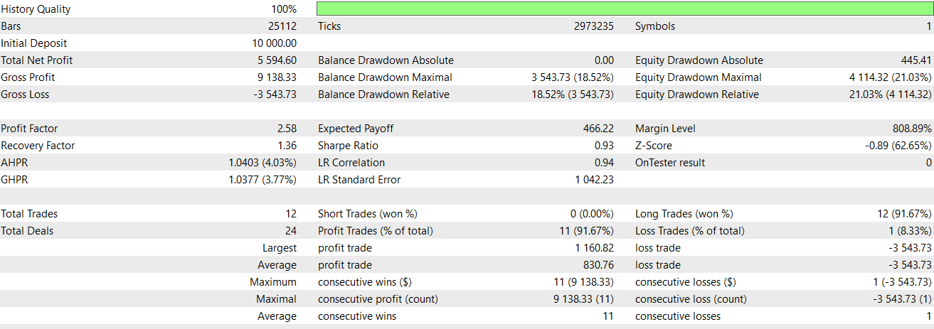
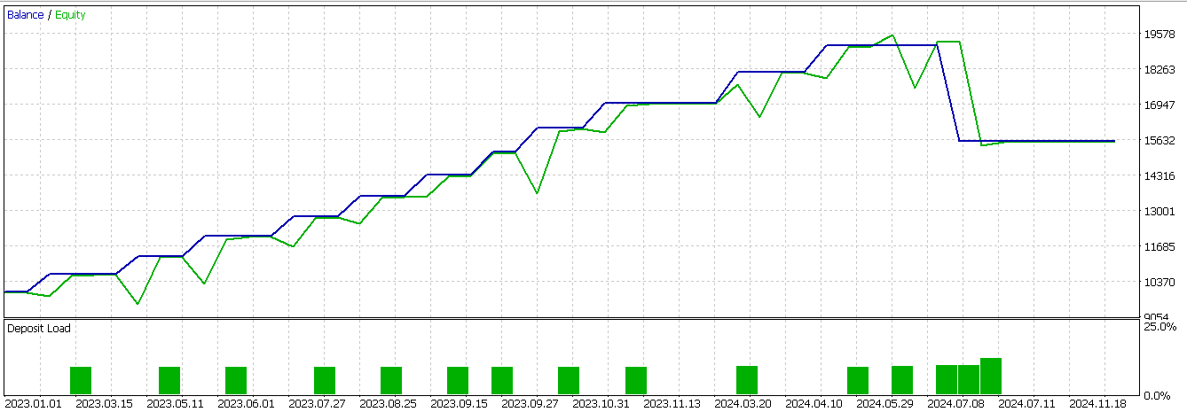
We perform optimizations and forward run tests for feature-4 when we supplement it with our CNN above as a filter. To recap from the last article, our symbol is USD JPY, the timeframe is 30-minute and as always, for this year at least, the test window is 2023 and 2024. Feature-4 is able to forward walk better, albeit with a loss, than what we had in the last article. This report is given below:

Feature-8

As covered in the last article, this signal pattern has a bullish signal of AO and price consistently rising, with AO above zero and price pulling away from the envelope lower band. The bearish logic has AO and price in a downward tear, with AO below zero, and price dropping off below the lower band. We implement this feature in Python as follows:

def feature_8(df):
    """
//+------------------------------------------------------------------+
//| Check for Pattern 8.                                             |
//+------------------------------------------------------------------+
    """
    feature = np.zeros((len(df), 2))
    
    feature[:, 0] = ((df['AO'].shift(2) > 0.0) &
                     (df['AO'].shift(1) > df['AO'].shift(2)) &
                     (df['AO'] > df['AO'].shift(1)) &
                     (df['close'].shift(2) > df['Envelope_Lower'].shift(2)) &
                     (df['close'].shift(1) > df['close'].shift(2)) &
                     (df['close'] > df['close'].shift(1))).astype(int)
    
    feature[:, 1] = ((df['AO'].shift(2) < 0.0) &
                     (df['AO'].shift(1) < df['AO'].shift(2)) &
                     (df['AO'] > df['AO'].shift(1)) &
                     (df['close'].shift(2) < df['Envelope_Lower'].shift(2)) &
                     (df['close'].shift(1) < df['close'].shift(2)) &
                     (df['close'] < df['close'].shift(1))).astype(int)
    
    
    feature[0, :] = 0
    feature[1, :] = 0
    
    return feature

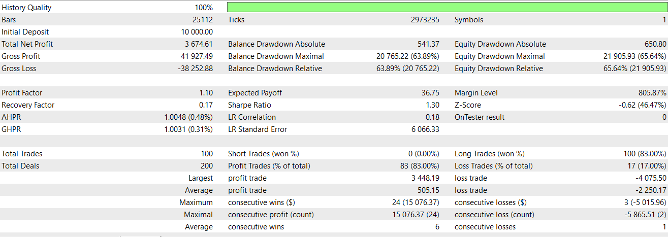
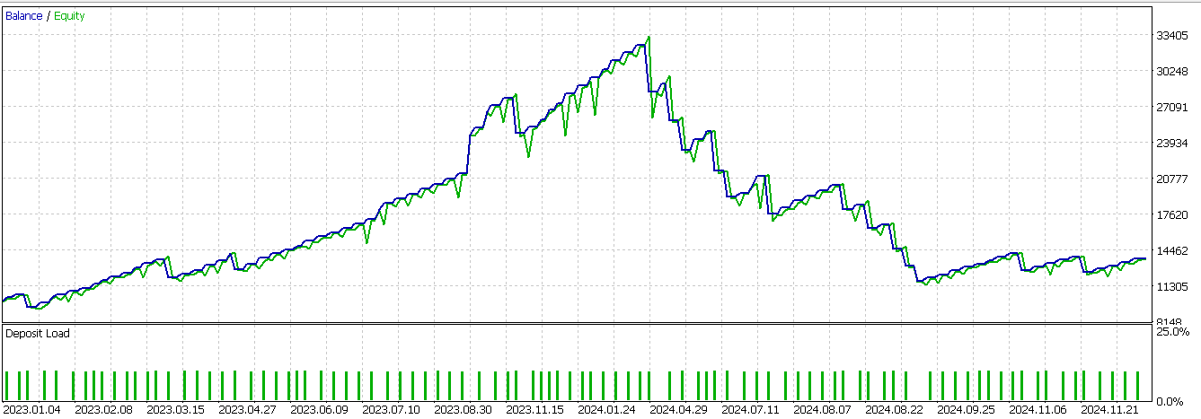
Therefore, from our code above, we give the first index a 1 confirming a bullish signal is present if the AO keeps moving up as well as price with clear acceleration from a positive zone. We also need to confirm that price is staying above the lower envelope and that this is not a dead cat bounce. The second index gets a 1 if AO starts negative having been dropping, but then ticks up potentially in a retracement, while price continues dropping in a strong downtrend below the lower envelope. We then do the zeroing of the first 2 indices as we did with feature-4. On testing feature-8, we still fail to get a profitable forward walk. This report is given below:

Feature-9

The core logic to our final signal pattern, as mentioned in the last article, is the AO rolling over but remaining above zero while price dips to the midline and bounces for the bullish signal. For the bearish signal, the AO is rolling up but remains below zero and price rallies to the midline, but then fails to surge beyond it. We implement it in Python as follows:

def feature_9(df):
    """
//+------------------------------------------------------------------+
//| Check for Pattern 9.                                             |
//+------------------------------------------------------------------+
    """
    feature = np.zeros((len(df), 2))
    
    feature[:, 0] = ((df['AO'].shift(2) > df['AO'].shift(1)) &
                     (df['AO'].shift(1) > df['AO']) &
                     (df['AO'] > 0.0) &
                     (df['close'].shift(2) > df['Envelope_Mid'].shift(2)) &
                     (df['close'].shift(1) <= df['Envelope_Mid'].shift(1)) &
                     (df['close'] > df['Envelope_Mid'])).astype(int)
    
    feature[:, 1] = ((df['AO'].shift(2) < df['AO'].shift(1)) &
                     (df['AO'].shift(1) < df['AO']) &
                     (df['AO'] < 0.0) &
                     (df['close'].shift(2) < df['Envelope_Mid'].shift(2)) &
                     (df['close'].shift(1) >= df['Envelope_Mid'].shift(1)) &
                     (df['close'] < df['Envelope_Mid'])).astype(int)
    
    
    feature[0, :] = 0
    feature[1, :] = 0
    
    return feature

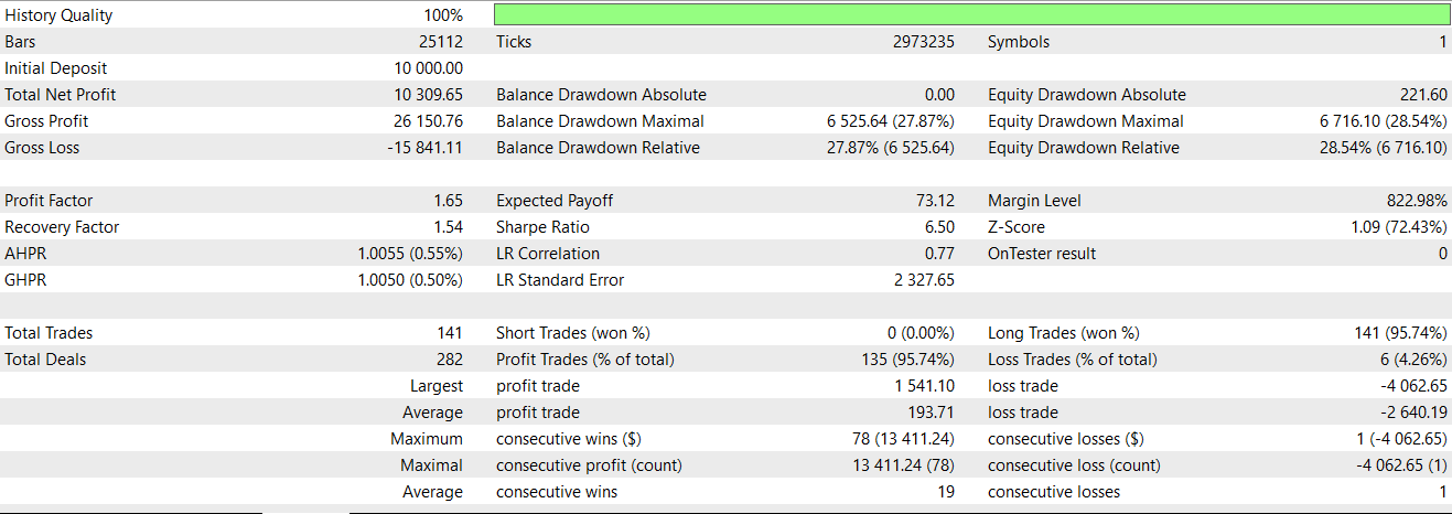
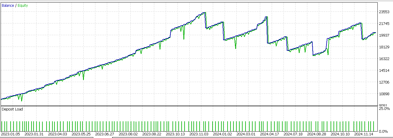
Our implementation ethos is in line with the two functions we have covered above so I will not reiterate the key points already covered. Testing our final pattern does give us an almost favourable forward walk. This report is shown below;

Conclusion

To sum up, we have explored the integration of machine learning, specifically through the use of a CNN as guided by a dot product kernel with cross time attention, to improve the signals of the AO and the envelope channels. Our test runs dwelt on the three previously tested patterns (pattern-4, pattern-8, and pattern-9) to establish if adding advanced neural filtering could enhance their forecasting performance.

Our dynamic CNN method did prove fruitful, particularly for the feature-4 and feature-9, where we turned what were previously woeful walk-forwards into runs where the losses were more contained. Our kernel’s attention mechanism allowed the network to dynamically adapt both kernel sizes and channel dimensions based on time relevance, which ended up capturing deeper patterns in market behaviour. This adaptability served us well since we are handling non-stationary financial markets. The case here being that rigid models usually underperform because of changes in either volatility, trend dynamics, or market regime.

However, not all results were positive. Feature-8 that relies a lot on sustained directional momentum did not achieve profitability even with the CNN’s improved adaptability. This suggests that certain signals are limited, regardless of model enhancements, highlighting the importance of indicator and signal selection in trading strategy. Besides supervised learning that we have explored in this article, we can revisit reinforcement learning as a means of improving our signals. In the next or future articles this could be explored for the features discussed here.

name	description
WZ-76.mq5	Wizard assembled Expert Advisor whose header highlights files included
SignalWZ-76.mqh	Custom Signal Class used by MQL5 Wizard in assembly
76-4.onnx	Exported Network for signal pattern-4
76-8.onnx	Exported network for signal pattern-8
76-9.onnx	Exported network for signal pattern-9