Money management in trading

Introduction

Money management is a very important aspect for successful trading. Its main purpose is to minimize risks and maximize profits. With the right use of money management, it is possible to achieve improved trading results.

In general, money management is a set of rules that allows traders to calculate the optimal volume of positions, taking into account all the possibilities and limitations. Today, there are quite a few money management strategies to fit every taste. We will try to consider several ways to manage money based on different mathematical growth models.

Trading strategy and money management

Any method of money management can accelerate the growth of the trading balance, or, in other words, to increase the profitability of the trading strategy. Thus, the trading strategy is the basis, while money management is an addition. Let's see what requirements a trading strategy must meet in order to apply money management to it.

First, it is the mandatory use of stop losses and take profits. With their help, you can control trading risks: stop loss allows you to limit possible losses, and take profit makes it possible to assess the potential profit for each deal.

Second, it is a positive mathematical expectation. It enables traders to evaluate the expected profitability of a trading strategy in the long term, which allows them to make rational decisions and manage their capital more efficiently. However, mathematical expectation is important not only for the trading strategy as a whole, but also for a newly opened position.

Let's introduce the following variables:

• p – probability of a profitable trade;
• SL – difference between the open price and stop loss in points;
• TP – difference between the open price and take profit.

First, we need to estimate the probability of profit. Let m be the number of closed profitable deals, while n is a total number of trades. Then the probability of receiving profit is:

The mathematical expectation (in points) for the position being opened can be found using the equation:

For a profitable trading strategy, the mathematical expectation should be positive. In this case, the use of any method of money management can bring additional profit.

However, the mathematical expectation may turn out to be negative or zero. This may happen at the very beginning of trading, when the number of losing trades can have a very large impact on the estimation of the profit probability. In this case, the volume of the opened position should be as small as possible. This means the trader needs to apply money management according to the linear growth model with minimal risk.

Linear growth

This is one of the most famous and simple growth patterns. Its use in trading is even simpler - a trader needs to choose a fixed position size and use it throughout the entire trading session. This model can be described using the linear function equation:

For convenience, convert this equation into a discrete form. Let deposit[i] be the value of the trading balance on the ith step. Then the linear balance growth equation will look like this:

where L is some constant that determines the rate of linear growth.

Let's rearrange this equation a bit. Let the res[i] variable will mark the results of the ith trade. Then we get the following equality:

Let's assume that we have n completed trades. Then we can use the least squares method to estimate the L value:

In this case, the L value will be equal to the arithmetic mean of the results of all deals.

However, the arithmetic mean can also provide an incorrect result. Let's assume that you have just started trading and there have been several losing trades. Then, the L value will be negative, and it will not be possible to use it in further calculations.

Let's introduce an additional condition – the L value should aim for the best possible one. Only if this condition is met, the deposit will grow at the maximum rate. Then we will use the following expression to evaluateL:

In this case, L will be equal to the mean square of the results of all trades. This estimate allows us to get the ideal linear growth rate, which will always be greater than the real growth rate of the deposit.

Now it is time to see how we can determine the optimal position size. Let's introduce the following variables:

• PV – price of one point in the deposit currency;
• Lot – position volume.

Let's find the L first:

The position may turn out to be profitable. Then its result will be Lot*TP*PV. Obviously, in this case, any trader will be interested in increasing the deposit growth rate and maximizing L. It can be expressed like this:

But the deal may also turn out to be unprofitable. Then the trader will try to avoid the loss leading to an increase in L:

Now we can combine both of these conditions and calculate the optimal position size:

We can make the model more versatile by adding risk to it. Let's add a new variable:

• R – parameter that determines the degree of risk.

Then, the expression for finding the optimal lot will look like this:

Thia means the trader should be prepared to lose a little more than is provided by the strict model. In this case, the optimal position size will be as follows:

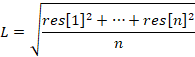
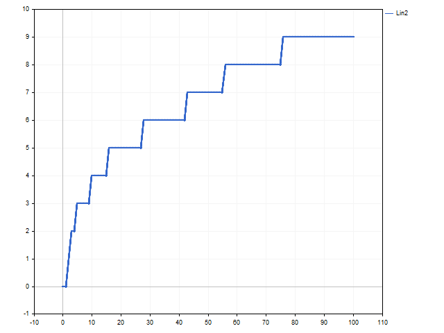
The R variable should be at least 1. The higher the variable, the higher the risk and the stronger the deviation from the linear growth model. This approach to money management may prove to be more attractive. For example, this is how the balance curve looks like when R = 3.

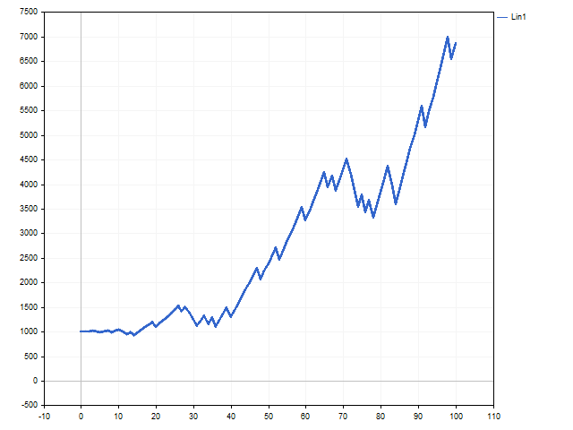
This is how the position volume changed. This chart shows by how many steps the minimum allowable position volume has been increased.

The increase in risk led to a rapid increase in the volume of positions. This made it possible to increase the initial capital by 7.5 times.

In addition, we can apply an empirical approach to the linear growth model. Let's rewrite the original lot calculation equation as follows:

That is, we explicitly indicate that the size of the position depends on two related factors - the possible loss and potential profit. There will be minimal losses only if a position with a minimum lot is opened. Let us denote the minimum position size of the lot variable and add the ability to manage risk. In this case, we get the following equation:

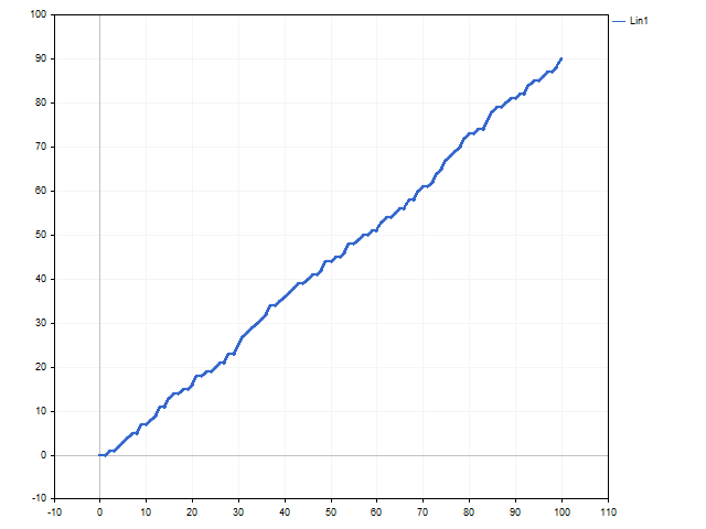
Note that the larger the R variable, the less the trading risk. This approach is a bit like the fixed-fractional method proposed by Ryan Jones in his book "The Trading Game. Playing by the Numbers to Make Millions". This method can be called linear growth with a gradual increase in speed. All depends on the L variable. As long as its value is stable, trading is carried out with a fixed lot. This is how the graphs of balance and position volume changes look like if R = 1.

Exponential growth

In everyday life, the "exponential growth" expression is most often used to refer to a very rapid increase in some parameter. Compound interest serves as an example of such growth. The exponential growth model in trading can be implemented using Kelly criterion and optimal f by Ralph Vince. The simplest implementation of this growth is trading with a fixed percentage. The trader only needs to find the optimal percentage for trading. Let's see how this can be done.

The discrete equation of exponential growth can be written as follows:

We can find the value of the growth parameter using the following equation:

In this case, the change in the trading balance can be described by the following equation:

It goes without saying that a trader is interested in obtaining the maximum end result. Let's see how we can achieve this.

First, we need to clear the result of each trade from the influence of the lot. To do this, we need to divide the obtained result by the deal volume:

In other words, Res[i] is a result of the ith trade in case its volume were equal to 1 lot.

Now we need to find such a position volume that the following condition is fulfilled:

But that is not all. Exponential growth can bring big gains, but losses can also be huge. To reduce the possible loss, we need to supplement the lot calculation with the possible results of a future deal. Then the volume of the future position can be calculated as follows. Let's find the sum first:

Then, the optimal volume for the opened position will be equal to:

Of course, this equation can be modified. For example, a trader may be cautious and assume the worst-case scenario of future events always expecting to lose. Then the equation for calculating the position volume will be as follows:

Here is an interesting feature. When considering linear growth models, we introduced risk at our discretion. Unlike that, in the exponential growth model, the risk appears as a result of a rigorous mathematical solution. The higher the R parameter, the lower the risk.

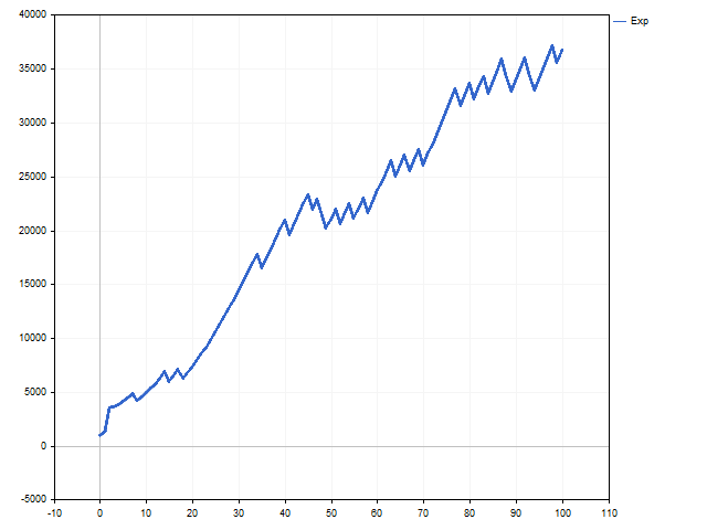
This is how the balance and lot curves look like in case of exponential growth.

Hyperbolic growth

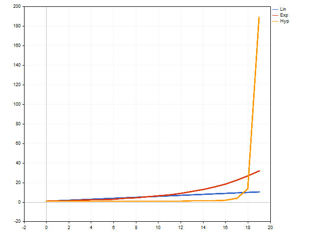
The main feature of hyperbolic growth is that it can reach an infinite value in a finite number of steps. Other models cannot boast of such a feature. Hyperbolic growth is very slow at first. It is too slow compared to exponential and even linear growth. But it is gaining momentum very quickly and there comes a moment when no one can catch up with it.

In general, the hyperbolic growth equation looks like this:

where N is a total number of model steps, while n is a number of steps already taken. The smaller the difference between them, the faster growth accelerates. If these parameters are equal, we get infinity.

Such an equation is not suitable for use in trading - we know neither the total number of steps, nor how many steps we have already passed. Fortunately, the discrete hyperbolic growth equation is free from these shortcomings:

Unfortunately, there are no easy ways to calculate the optimal position size. For calculations, we will have to use numerical methods.

First, assign the minimum value to the Lot variable and find the value of the sum: 

Now let's take into account the possible options for the position being opened and get the final value:

Save the absolute value D. Then increase the Lot variable one step and repeat the calculations from the beginning. If the new value D turned out to be less than the previous one, then it is necessary to increase the Lot variable again and repeat the calculations. If the D value is higher than the previous one, the calculations are stopped. The optimal position volume will be equal to the Lot variable obtained at the previous step.

The use of the hyperbolic growth model is associated with a very high risk. In order to reduce it, we can use the R variable. The higher it is, the lower the risk. Of course, we can prepare for a loss in advance. Then D is calculated using the following equation:

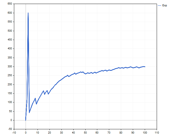
This is how the balance change according to the hyperbolic law looks like.

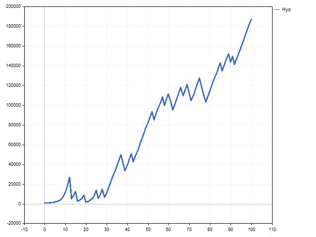
Now it is time for a surprise. Look at the volume change graph. We see that after the 30th deal, the lot becomes fixed. It may seem that the hyperbolic growth has been replaced by the linear one.

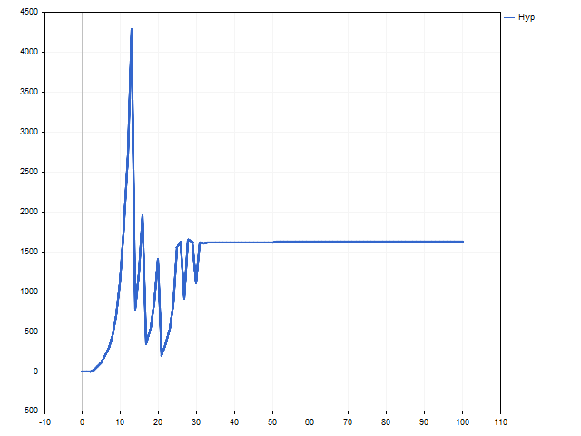
This is a normal behavior for the hyperbolic growth model. It is too perfect for the real world - the trading balance cannot grow indefinitely. In this case, we can say that the model decided that the hyperbolic growth is at the very beginning, so the change in the volume of positions became small. Whether we can see an ascending branch of hyperbolic growth depends on the trading strategy and luck.

Conclusion

So, we got acquainted with the basic mathematical models of growth. Now let's see if these models can be applied in practice.

Considering margin requirements is a must here. The model may suggest a position volume that is larger than the allowable one.

In addition, the trading strategy may turn out to be asymmetric in the direction of deals. For example, Buy positions may be more profitable than Sell positions. In this case, the lot calculation should depend on the type of a position being opened.

Now let's look at the results we can expect in the market conditions. To do this, we will write a simple Expert Advisor that opens positions when simple moving averages cross. Positions are closed when the stop loss or take profit is reached. MinLot money management — all positions are opened with a minimum volume. Below are the EA testing parameters.

• Symbol: EURUSD
• Timeframe: H1
• Test period: 2021.01.01 - 2022.12.31
• Initial deposit: 10,000
• Total trades: 509

Money Management	Risk	Total Net Profit	Gross Profit	Gross Loss	Profit Factor	Expected Payoff
MinLot	-	466.70	2 119.92	-1 653.22	1.28	0.92
Lin1	7	39 593.81	190 376.71	-150 782.90	1.26	77.79
Lin2	1	1 719.91	7 625.00	-5 905.09	1.29	3.38
Exp	3	12 319.19	77 348.22	-65 029.03	1.19	24.20
Hyp	5	24 946.38	100 778.15	-75 831.77	1.33	49.01

Of course, pay attention to how risk affects return.

Programs that were used when writing the article.

Name	Type	Features
Money Management	script	The script simulates money management. ProbabilityWin - profit probability Trades - number of simulated trades StartDeposit - initial deposit SL & TP - stop loss and take profit of deals Risk - risk value Lin1 ... Hyp - money management type ScreenShot - saves the graph in the Files folder
Growth	script	Shows the difference between linear, exponential and hyperbolic growth.
EA Money Management	EA	Only for testing different money management methods. MoneyManagement - selecting a money management method Risk - acceptable risk SL & TP - stop loss and take profit of positions PeriodMA1 & PeriodMA2 - moving average periods