Singular Spectrum Analysis in MQL5

What is SSA?

Recent iterations of MetaTrader 5 have introduced the initial integration of OpenBLAS methods into its core vector and matrix data types. Of particular interest are a set of methods related to Singular Spectrum Analysis (SSA). In this article, we explore the new tools available in MQL5 related to SSA and unpack how they can be used in analysis and forecasting. This guide aims to provide a resource for traders seeking to harness SSA's full potential. We will delve into the core SSA methodology, demystifying its two-stage decomposition and reconstruction process. More importantly, we will discuss what each of the new SSA vector methods do and demonstrate how to interpret and optimally combine their outputs for actionable insights.

Singular Spectrum Analysis is a non-parametric technique designed for the analysis and forecasting of time series data. Its objective is to decompose a time series into a few additive components, which typically include a slowly varying trend, various cycles, and residual noise. A distinguishing feature of SSA is its minimal reliance on predetermined assumptions regarding the underlying data-generating process. The conceptual foundation of SSA integrates elements from statistics and signal processing. Essentially, SSA is rooted in spectral decomposition, allowing it to reveal the frequency characteristics of a time series by analyzing its principal components in a reconstructed embedding space. It can be effectively conceptualized as a form of Principal Component Analysis (PCA) specifically adapted for time series data, leveraging the principles of dimensionality reduction to uncover hidden structures and patterns that might be obscured by noise or complex interactions.

SSA in MQL5

In MQL5, SSA calculations are implemented natively as methods of the vector data type and also in the Alglib math library. The strength of the Alglib implementation of SSA is primarily in real-time processing, while the new SSA functionality directly accessible from vectors is more suitable for exploratory analysis. Note that while this text is primarily concerned with operations using real numbers, equivalent methods for complex numbers are also available and work similarly, with their interpretation tailored for the complex domain.

In each of the new vector SSA methods, the first required parameter is the specification of a window length. This parameter dictates how the time series is transformed into a higher-dimensional structure known as the trajectory matrix. One may be asking, "Why the need for this higher-dimensional structure?" The clue lies in SSA's relation to PCA. Remember, PCA is a dimensionality reduction technique employed on multivariate datasets. SSA reconstructs a univariate time series into a structure that resembles a multivariate dataset. This is done by arranging sections of the series in rows of equal size. Here, the size of a row is defined by the window length parameter.

Consider a time series Y=[y1​,y2​,y3​,y4​,y5​,y6​] of length N=6. If a window length of L=3 is chosen, it results in a trajectory matrix equivalent to the one below.

The number of rows, R, in the matrix is calculated as R=N−L+1. In this example, R=6−3+1=4. This matrix, of dimension R×L (in our example, 4×3), is the trajectory matrix. The patterns observed on the anti-diagonals of this matrix are characteristic of a Hankel matrix. The construction of the trajectory matrix is the first step of the SSA method. It comes as no surprise, then, that the window length is a defining parameter of the SSA method, as it directly determines the dimensions of the trajectory matrix, which in turn significantly affects the resolution and separability of the spectral decomposition.

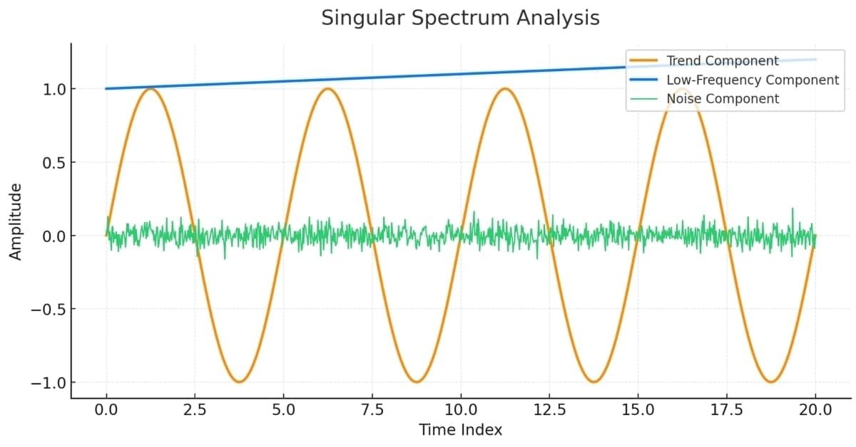
To elucidate the concepts of SSA methodology, we will demonstrate its application to a deterministic series, which is depicted below.

This series was constructed from predetermined additive components consisting of a trend, a couple of periodic components, and random noise. When these components are added together, the result is a somewhat irregular series. The goal of SSA is to uncover these underlying components. This is done by decomposing either the trajectory matrix or the covariance matrix of the trajectory matrix, yielding the eigenmodes, which, as in PCA, reveal the principal components of the series.

Relative and Cumulative Component Contributions

The MQL5 vector method, SingularSpectrumAnalysisSpectrum(), outputs a vector representing the relative component contributions of a series. This vector contains real numbers that sum to one, indicating the fractional dominance of each component, arranged in descending order. These contributions correspond to relative magnitudes of the eigenvalues calculated by the decomposition of a matrix.

//---
   vector relative_contributions;
   if(!full_process.SingularSpectrumAnalysisSpectrum(WindowLen,relative_contributions))
     {
      Print(" error ", GetLastError());
      return;
     }
//---
   relative_contributions*=100.0;
   vector cumulative_contributions = relative_contributions.CumSum();

When the cumulative sum of the relative contributions is calculated, we get the cumulative contributions. These values allow us to quickly ascertain the fewest number of components required to achieve a relatively close approximation of the original series. A plot of the relative contributions often exhibits distinct approximate plateaus, suggesting that some component contributions are similar in value. This similarity typically indicates that these components may represent a single periodic element.

Below are the relative and cumulative contribution plots for our example series.

These show that the first two components contribute about 68% and 12% of the total variance in the series.

The first five components alone account for over 98%. The plot of the relative contributions carves out a unique shape that exposes the dominance of the first 5 components. The point that separates the dominant components from the rest is usually referred to as the "elbow point," and the components below this level are called the "noise floor." It provides a rough estimate of the separation of the signal from the noise. Another notable aspect of the relative contributions plot is how components number two and three are grouped together away from the fourth and fifth components. This gives an indication that these paired groups are related and may represent unique features of the series.

Extraction of Series Components

Having analyzed our example series, we now have an understanding of the major components that define the bulk of its behavior. To assess their regularity, it may be beneficial to visualize these components. This is where the vector method SingularSpectrumAnalysisReconstructComponents() proves useful. The output of particular interest is the matrix of component series. Be aware, however, that while the MQL5 documentation suggests the columns represent the estimated component series, the method actually stores each component series as a row in the matrix. Additionally, the method's vector output contains the raw eigenvalues of the decomposition of the representative matrix of the series.

//---
   matrix components;
   vector eigvalues;
   if(!full_process.SingularSpectrumAnalysisReconstructComponents(WindowLen,components,eigvalues))
     {
      Print(" error ", GetLastError());
      return;
     }
//---

The rows of the matrix of component series are arranged in decreasing order of relative contribution magnitude. Consequently, the first row contains the component corresponding to the largest eigenvalue, which also represents the component with the highest relative contribution. Below is a plot showing all the components of our example series.

If you compare this to a plot of the original components, you might notice some discrepancies. This highlights the fact that SSA decomposition is not exact. The method will never be able to decipher the exact periodic components of a series. All it can do is find optimal approximations or estimates of these components. Nevertheless, summing the separate component series will result in the original series.

Filtering

With the set of component series in hand, we can use the information from SSA analysis to infer which components describe the underlying signal and which represent non-deterministic noise. If our primary concern is dominant cycles, we can discard components with lower relative contributions to produce a filtered series. By doing so, we assume these lesser components represent noise that obscures the main signal.

Users can perform this filtering directly on a series using the SingularSpectrumAnalysisReconstructSeries() method. A user specifies the number of dominant components to include in the filtered series.

//---
   vector filtered;
   if(!full_process.SingularSpectrumAnalysisReconstructSeries(WindowLen,FilterComponents,filtered))
     {
      Print(" error ", GetLastError());
      return;
     }

The SSA method is generally adept at isolating noise, but its effectiveness depends on the nature of the noise present in the process. Simply discarding components with lower relative contributions may not be sufficient for definitively isolating noise. Consequently, this also has an impact on the extraction of signals, trends, or specific periodic components. Interpretation of these components often needs to be validated by statistical tests of significance. Another aspect that may affect the isolation of specific components arises from the presence of strong trends, whose dominance may mask other low-frequency oscillations in the data.

Forecasting

One of the more interesting aspects of SSA methodology is its application to prediction. This functionality is provided by the SingularSpectrumAnalysisForecast() method. Once the time series has been decomposed and reconstructed, the forecasting step typically utilizes a recurrent forecasting algorithm. This algorithm leverages the inherent Linear Recurrent Relation (LRR) that the reconstructed components often satisfy. It is assumed that these reconstructed components follow a predictable pattern. Based on the singular vectors and the reconstructed series, a set of coefficients is determined. These coefficients represent the linear relationship between past and future values within the reconstructed signal. To forecast a new data point, the algorithm applies a linear combination of the previous 'window length' values of the reconstructed series, weighted by the determined coefficients. This process is then repeated iteratively to generate multiple forecasts.

//---
   vector forecast;
   if(!full_process.SingularSpectrumAnalysisForecast(WindowLen,FilterComponents,ForecastLen,forecast))
     {
      Print(" error ", GetLastError());
      return;
     }
//---

It should be obvious that such forecasts assume that previous patterns will manifest in the future exactly as they did in the past. Of course, this is unlikely to be true of real-world time series. Despite this, SSA can be useful in making complex processes more predictable by focusing on certain components with regular waveforms.

Parameter Selection and Preprocessing

It has already been established that decomposition of series with SSA will never be able to extract the exact periodic components of a time series. All it can do is extract estimates of the components. This is an obvious limitation of the method, which is further exacerbated by the method's sensitivity to the selected window length. Choosing the right window length can be guided by the goals of decomposition. If interest primarily lies in isolating the trend, then the larger the window length, the better. If, however, oscillatory components are of more importance, practitioners should consider the periods of oscillation; for example, if looking for a periodic component that oscillates with a period of 20, then set the window length to 20.

Empirical evidence presented in academic literature seems to suggest that the window length corresponds to the resolution of oscillations with periods in the range L/5 to L, where L is the window length. The problem is that the period of the component of interest may not be known beforehand, so a lot of trial and error is necessary. The general rule of thumb is to set the window length to between two and half the length of the series being studied. A longer window length amplifies the slower varying components, while smaller window lengths capture finer details.

Besides SSA's sensitivity to window length, practitioners should also know how strong trends present in time series may affect the results of decomposition. Strong trends can mask other low-frequency components in the series. This problem can be primarily dealt with by detrending the raw series before applying SSA. Types of preprocessing that can be applied include centering or removing the linear trend, as shown in the code snippet below.

//---
   if(m_detrend)
     {
      vector reg = m_buffer.LinearRegression();
      m_buffer -= reg;
     }
//---

When it comes to deciding how many components to select when filtering or forecasting, plots of relative and cumulative contributions can be of great help. The feature to identify on a plot of relative contributions is the "elbow" point, distinguishing the signal from the noise. The points on the plot associated with a signal will appear above a clear break from points whose values slowly decrease towards zero. The same should be visible when examining the decay of the raw eigenvalues of the decomposition process. Another viable option is to specify a target for the total percentage of variance to be captured, usually 85% to 95%, and then get the number of components that value corresponds to, within the series of cumulative contributions.

Component Grouping

We know that SSA decomposition will not magically reproduce the exact underlying components of a series; we have seen this with a simple example. What we get are a set of components that approximate the actual constituent series. We only have to figure out how to combine our estimates to get a better picture of the actual elements that define the process. This can be achieved by constructing the weighted correlation matrix of the component series. The weighted correlation matrix measures how a pair of component series differ from perfect orthogonality. If a pair of series components are perfectly orthogonal, then they are likely distinct components.

Higher correlations indicate that a pair should be combined. The code snippet below depicts a routine that calculates the weighted correlation matrix given a matrix of component series and the window length parameter of the SSA decomposition. The function is declared in ssa.mqh, which is attached to the article. 

//+------------------------------------------------------------------+
//| component correlations                                           |
//+------------------------------------------------------------------+
matrix component_corr(ulong windowlen,matrix &components)
  {
   double w[];
   ulong fsize = components.Cols();
   ulong r = fsize - windowlen + 1;
  
   for(ulong i = 0; i<fsize; i++)
     {
      if(i>=0 && i<=windowlen-1)
         w.Push(i+1);
      else
         if(i>=windowlen && i<=r-1)
            w.Push(windowlen);
         else
            if(i>=r && i<=fsize-1)
               w.Push(fsize-i);
     }

   vector weights;
   weights.Assign(w);
   ulong d = windowlen;

   vector norms(d);
   matrix out = matrix::Identity(d,d);

   for(ulong i = 0; i<d; i++)
     {
      norms[i] = weights.Dot(pow(components.Row(i),2.0));
      norms[i] = pow(norms[i],-0.5);
     }

   for(ulong i = 0; i<d; i++)
     {
      for(ulong j = i+1; j<d; j++)
        {
         out[i][j] = MathAbs(weights.Dot(components.Row(i)*components.Row(j))*norms[i]*norms[j]);
         out[j][i] = out[i][j];
        }
     }

   return out;
  }

A section of the component correlations that make up the top six components of our example series is shown below.

The graphic shows the high correlation between components at index (1:2), which corresponds with components 2 and 3 being related, while components referenced at index (3:4) refer to the relation between components 4 and 5. This analysis seems to agree with the visual inspection of the relative contributions plot seen earlier. From here, we could then hypothesize that the two groups of components may point to the periodic components of our example series. The single topmost component is distinct and likely the trend. As we already saw from the cumulative contributions, these 5 components account for 98% of contributions; the rest is therefore likely noise.

Viewing Price Series Decompositions

In this section, we present an application implemented as an Expert Advisor that can be used to view the components of an arbitrary sample of prices. The application has a graphical user interface that allows users to set the symbol, date, and length of the price series to display and decompose. There is an option to detrend the series before decomposition. The relative and cumulative contribution plots can be optionally viewed as well. Below is a screenshot of the application displaying a sample of EURUSD close prices, with a decomposed component shown on the plot at the bottom.

Conclusion

This article explored the new MQL5 tools for Singular Spectrum Analysis (SSA), highlighting the OpenBLAS additions to the vector data type. We provided a concise overview of the SSA method, intentionally avoiding in-depth mathematical explanations. In summary, SSA is a valuable tool for any practitioner, but it requires careful parameter selection and an understanding of its operational nuances to be fully effective. All referenced code is included and attached below. 

File Name	File Description
MQL5/include/ssa.mqh	This header file contains the definition of the function the implements the calculation component correlations described in the section titled Component Grouping.
MQL5/scripts/SSA_Filtered_Demo.mq5	This is the script used to demonstrate filtering with SSA.
MQL5/scripts/SSA_Decomposition_Demo.mq5	This is the script used to demonstrate the decomposition of a series with SSA.
MQL5/scripts/SSA_ComponentContributions_Demo.mq5	This is the script used to demonstrate the display of relative component contributions.
MQL5/scripts/SeriesPlot.mq5	This script was used to plot the different components of the example series referenced in the article.
MQL5/experts/SSA_PriceDecomposition.ex5	This EA is a program that can be used to display the decomposition of an arbitrary price series.
MQL5/experts/SSA_PriceDecomposition.mq5	This is the source code for the EA listed above.