
数据科学和机器学习(第 30 部分):预测股票市场的幂对、卷积神经网络(CNN)、和递归神经网络(RNN)

内容
概述
在之前的文章中,我们已见识到卷积神经网络(CNN)和递归神经网络(RNN)的强大功能,以及如何部署它们,通过提供有价值的交易信号来帮助我们抗击市场。
在本篇中,我们将尝试组合 CNN 和 RNN 这两种最强大的技术,并观察它们对股票市场的预测影响。但在此之前,我们简要了解 CNN 和 RNN 的全部内容。
了解递归神经网络(RNNs)和卷积神经网络(CNNs)
卷积神经网络(CNN)旨在识别数据中的形态和特征,尽管最初是为图像识别任务开发的,但它们依据专为时间序列预测设计的表格数据中表现优良。
如前几篇文章所述,它们的工作原理是首先对输入数据应用过滤器,然后提取可用于预测的高级特征。在股票市场数据中,这些特征包括趋势、季节性影响、和异常。

CNN 架构
借力 CNN 的层次化性质,我们可以揭示数据表示层,每层都针对市场不同方面提供了见解。
递归神经网络(RNN)是人工神经网络,旨在识别数据序列中的形态,例如时间序列、语言、或视频。
与传统神经网络不同,其假设输入彼此独立,而 RNN 能从一系列数据(信息)中检测和理解形态。
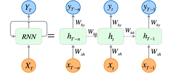
RNN 是专门为顺序数据设计的,它们的架构允许它们保持对先前输入的记忆,这令它们非常适于时间序列预测,因为理解数据中时态依赖关系的能力,对于在股票市场做出准确预测至关重要。
正如我在本系列的第 25 部分中所解释的那样,有三种(常用的)特定类型的 RNNs,包括原版的递归神经网络(RNN)、长短期记忆(LSTM)、和门控递归单元(GRU)。
由于 CNNs 擅长从数据中提取和检测特征,故 RNN 在随时间推移解释这些特征方面非常出色。该思路很简单,将这两者结合起来,看看我们能否构建一个强大而健壮的模型,能够在股票市场做出更好的预测。
CNN 和 RNN 的协同
为了集成这两者,我们将分三个步骤创建模型。
- 配合 CNN 特征提取
- 配合 RNN 时态建模
- 训练和获取预测
我们会一步步构建这个由 RNN 和 LSTM 组成的健壮模型。
01:配合 CNNs 提取特征
第一步涉及将时间序列数据馈送到 CNN 模型之中,CNN 模型处理数据,识别重要形态、并提取相关特征。
使用 Tesla 股票数据集,其由开盘价、最高价、最低价、和收盘价组成。我们首先准备数据,即 CNNs 和 RNNs 可接受的 3D 时间序列格式。
我们为分类问题创建目标变量。
Python 代码
target_var = []

open_price = new_df["Open"]
close_price = new_df["Close"]

for i in range(len(open_price)):
    if close_price[i] > open_price[i]: # Closing price is greater than opening price
        target_var.append(1) # buy signal
    else:
        target_var.append(0) # sell signal
我们使用 标准伸缩器 对数据进行归一化,令其针对 ML 目的更健壮。
X = new_df.iloc[:, :-1]
y = target_var

# Scalling the data

scaler = StandardScaler()
X = scaler.fit_transform(X)

# Train-test split

X_train, X_test, y_train, y_test = train_test_split(X, y, test_size=0.2, shuffle=False)

print(f"x_train = {X_train.shape} - x_test = {X_test.shape}\n\ny_train = {len(y_train)} - y_test = {len(y_test)}")
输出
x_train = (799, 3) - x_test = (200, 3)

y_train = 799 - y_test = 200
然后,我们准备数据,按时间序列格式。
# creating the sequence

X_train, y_train = create_sequences(X_train, y_train, time_step)
X_test, y_test = create_sequences(X_test, y_test, time_step) 由于这是一个分类问题,故我们对目标变量进行独热编码。
from tensorflow.keras.utils import to_categorical

y_train_encoded = to_categorical(y_train)
y_test_encoded = to_categorical(y_test)

print(f"One hot encoded\n\ny_train {y_train_encoded.shape}\ny_test {y_test_encoded.shape}")
输出
One hot encoded

y_train (794, 2)
y_test (195, 2)
特征提取由 CNN 模型本身执行,我们给出刚刚准备好的模型原生数据。
model = Sequential()
model.add(Conv1D(filters=16,
                 kernel_size=3,
                 activation='relu',
                 strides=2,
                 padding='causal',
                 input_shape=(time_step, X_train.shape[2])
                )
         )

model.add(MaxPooling1D(pool_size=2))
02:配合 RNNs 时态建模
然后,将上一步中提取的特征传递至 RNN 模型。该模型处理这些特征时,会参考数据中的时态顺序和依赖关系。
与本系列文章第 27 部分中用到的 CNN 模型架构不同,我们在 “Flatten layer” 之后使用了全连接神经网络层。这次,我们将这些常规神经网络(NN)层替换为递归神经网络(RNN)层。
不要忘记删除 CNN 架构图片中看到的 “Flatten layer”。
我们删除了 CNN 架构中的 Flatten 层,因为该层通常将 3D 输入转换为 2D 输出,而 RNN(RNN、LSTM 和 GRU)需要 3D 输入数据,其形式为(批次大小、时间步长、特征)。
model.add(MaxPooling1D(pool_size=2))

model.add(SimpleRNN(50, activation='relu'))
model.add(Dropout(0.5))
model.add(Dense(50, activation='relu'))
model.add(Dropout(0.5))
model.add(Dense(units=len(np.unique(y)), activation='softmax'))  # Softmax for binary classification (1 buy, 0 sell signal)
03: 训练和获取预测
最后,我们可以继续训练我们在前两步中构建的模型,然后,我们验证它,衡量其性能,然后从中得出预测。
Python 代码
model.summary()

# Compile the model
optimizer = Adam(learning_rate=0.0001)
model.compile(optimizer=optimizer, loss='binary_crossentropy', metrics=['accuracy'])

# Train the model
early_stopping = EarlyStopping(monitor='val_loss', patience=10, restore_best_weights=True)

history = model.fit(X_train, y_train_encoded, epochs=1000, batch_size=16, validation_split=0.2, callbacks=[early_stopping])

plt.figure(figsize=(7.5, 6))
plt.plot(history.history['loss'], label='Training Loss')
plt.plot(history.history['val_loss'], label='Validation Loss')
plt.xlabel('Epochs')
plt.ylabel('Loss')
plt.title('Training Loss Curve')
plt.legend()
plt.savefig("training loss curve-rnn-cnn-clf.png")
plt.show()

# Evaluating the Trained Model

y_pred = model.predict(X_test)


classes_in_y = np.unique(y)
y_pred_binary = classes_in_y[np.argmax(y_pred, axis=1)]

# Confusion Matrix
cm = confusion_matrix(y_test, y_pred_binary)
sns.heatmap(cm, annot=True, fmt='d', cmap='Blues')
plt.xlabel("Predicted Label")
plt.ylabel("True Label")
plt.title("Confusion Matrix")
plt.savefig("confusion-matrix RNN + CNN.png")  # Display the heatmap


print("Classification Report\n",
      classification_report(y_test, y_pred_binary))
输出
经历 14 个局次后评估模型,该模型在测试数据上的准确率为 54%。

7/7 ━━━━━━━━━━━━━━━━━━━━ 0s 33ms/step
Classification Report
               precision    recall  f1-score   support

           0       0.70      0.40      0.51       117
           1       0.45      0.74      0.56        78

    accuracy                           0.54       195
   macro avg       0.58      0.57      0.54       195
weighted avg       0.60      0.54      0.53       195
值得一提的是,当添加更多层时,训练最终模型需要一些时间,这是由于我们组合两个模型的复杂性。
训练后,我必须将最终模型保存为 ONNX 格式。
Python 代码
onnx_file_name = "rnn+cnn.TSLA.D1.onnx"

spec = (tf.TensorSpec((None, time_step, X_train.shape[2]), tf.float16, name="input"),)
model.output_names = ['outputs']

onnx_model, _ = tf2onnx.convert.from_keras(model, input_signature=spec, opset=13)

# Save the ONNX model to a file
with open(onnx_file_name, "wb") as f:
    f.write(onnx_model.SerializeToString())
不要忘记保存标准化伸缩器参数。
# Save the mean and scale parameters to binary files

scaler.mean_.tofile(f"{onnx_file_name.replace('.onnx','')}.standard_scaler_mean.bin")
scaler.scale_.tofile(f"{onnx_file_name.replace('.onnx','')}.standard_scaler_scale.bin")
我在 Netron 中打开所保存 ONNX 模型,这是一个巨大的模型。

类似于我们之前部署卷积神经网络(CNN)所做,我们可调用相同函数库来帮助我们在 MQL5 中轻松读取这个庞大的模型。
#include <MALE5\Convolutional Neural Networks(CNNs)\ConvNet.mqh>
#include <MALE5\preprocessing.mqh>

CConvNet cnn;
StandardizationScaler *scaler; //from preprocessing.mqh
但是,在此之前,我们必须将 ONNX 模型和标准化伸缩器参数添加到我们的智能系统当中,作为资源。
#resource "\\Files\\rnn+cnn.TSLA.D1.onnx" as uchar onnx_model[]
#resource "\\Files\\rnn+cnn.TSLA.D1.standard_scaler_mean.bin" as double standardization_mean[]
#resource "\\Files\\rnn+cnn.TSLA.D1.standard_scaler_scale.bin" as double standardization_std[]
在 OnInit 函数中,我们要做的第一件事是初始化它们(标准化伸缩器和 CNN 模型)。
int OnInit()
  {
//---

   if (!cnn.Init(onnx_model)) //Initialize the Convolutional neural network
     return INIT_FAILED;

   scaler = new StandardizationScaler(standardization_mean, standardization_std); //Initialize the saved scaler by populating it with values

   ...
   ...

  return (INIT_SUCCEEDED);
 }
为了得到预测结果,我们须用这个预加载的伸缩器对输入数据进行归一化,后将归一化数据应用于 CNN 模型,并获得预测信号和概率。
   if (NewBar()) //Trade at the opening of a new candle
    {
      CopyRates(Symbol(), PERIOD_D1, 1, time_step, rates);

      for (ulong i=0;  i<x_data.Rows(); i++)
        {
          x_data[i][0] = rates[i].open;
          x_data[i][1] = rates[i].high;
          x_data[i][2] = rates[i].low;
        }

   //---

      x_data = scaler.transform(x_data); //Normalize the data

      int signal = cnn.predict_bin(x_data, classes_in_data_); //getting a trading signal from the RNN model
      vector probabilities = cnn.predict_proba(x_data);  //probability for each class

      Comment("Probability = ",probabilities,"\nSignal = ",signal);
下面是图表上的注释样子。

概率向量取决于您的训练数据中目标变量中存在的分类。依据训练数据,我们准备了目标变量,指示 0 代表卖出信号,1 代表买入信号。类标识符、或数字必须按升序排列。
input int time_step = 5;
input int magic_number = 24092024;
input int slippage = 100;

MqlRates rates[];
matrix x_data(time_step, 3); //3 columns for open, high and low
vector classes_in_data_ = {0, 1}; //unique target variables as they are in the target variable in your training data
int OldNumBars = 0;
//+------------------------------------------------------------------+
//| Expert initialization function                                   |
//+------------------------------------------------------------------+
int OnInit()
  {
//---
名为 x_data 的矩阵负责临时存储来自市场的自变量(特征)。由于我们依据 3 个特征(Open、High 和 Low)上训练模型,故该矩阵的大小被调整为 3 列,并调整到等于时间步骤值的行数。
时间步骤值必须与创建顺序训练数据时所用的时间步骤值相似。
我们可基于我们所构建模型提供的信号制定一个简单的策略。
   double min_lot = SymbolInfoDouble(Symbol(), SYMBOL_VOLUME_MIN);

      MqlTick ticks;
      SymbolInfoTick(Symbol(), ticks);

      if (signal==1) //if the signal is bullish
       {
          ClosePos(POSITION_TYPE_SELL); //close sell trades when the signal is buy

          if (!PosExists(POSITION_TYPE_BUY)) //There are no buy positions
           {
             if (!m_trade.Buy(min_lot, Symbol(), ticks.ask, 0 , 0)) //Open a buy trade
               printf("Failed to open a buy position err=%d",GetLastError());
           }
       }
      else if (signal==0) //Bearish signal
        {
          ClosePos(POSITION_TYPE_BUY); //close all buy trades when the signal is sell

          if (!PosExists(POSITION_TYPE_SELL)) //There are no Sell positions
           {
            if (!m_trade.Sell(min_lot, Symbol(), ticks.bid, 0 , 0)) //open a sell trade
               printf("Failed to open a sell position err=%d",GetLastError());
           }
        }
      else //There was an error
        return;
现在我们已加载了模型,并准备进行预测,我运行的测试介于 2020.01.01 到 2024.09.01 之间。下面是完整的测试器配置(settings)图片。
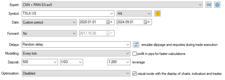
注意,我收集特斯拉股票数据时,在 4 小时图上应用 EA,取代日线时间帧。这是因为我们将策略和模型程序化,在新蜡烛开立后立即开始动作,但是,日线蜡烛通常在市场收市时才开立,故导致 EA 错过交易,直到第二天。
通过将 EA 应用于较低的时间帧(在本例中为 4 小时),我们确保每 4 小时后持续监控市场,并执行一些交易活动。
这不会影响提供给 EA 的数据,故我们在日线时间帧(交易决策仍然取决于日线图)调用 CopyRates 函数。
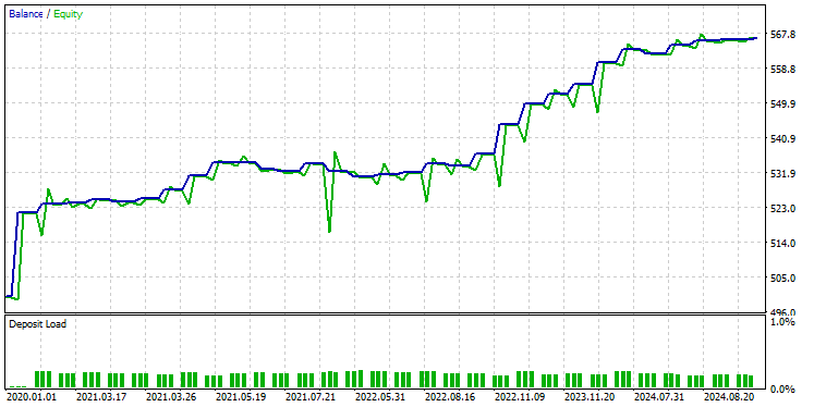
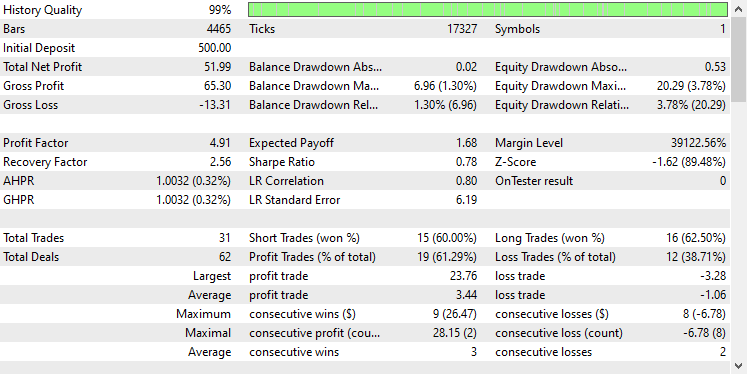
以下是测试器的结果。
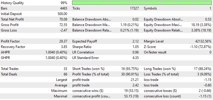
印象深刻!EA 产生了 90% 的盈利交易。AI 模型只是一个简单的 RNN。
现在我们看看 LSTM 和 GRU 在同一市场中的表现如何。
组合卷积神经网络(CNN)和长短期记忆(LSTM)
与简单的 RNN 不同,简单的 RNN 无法理解长期序列数据、或信息中的形态,而 LSTM 可以理解长期序列信息中的关系和形态。
LSTM 往往比简单的 RNN 更高效、更准确。我们创建一个包含 LSTM 的 CNN 模型,然后观察它在特斯拉股票中的表现。
Python 代码
from tensorflow.keras.layers import LSTM

# Define the CNN model

model = Sequential()
model.add(Conv1D(filters=16,
                 kernel_size=3,
                 activation='relu',
                 strides=2,
                 padding='causal',
                 input_shape=(time_step, X_train.shape[2])
                )
         )

model.add(MaxPooling1D(pool_size=2))


model.add(LSTM(50, activation='relu'))
model.add(Dropout(0.5))
model.add(Dense(50, activation='relu'))
model.add(Dropout(0.5))
model.add(Dense(units=len(np.unique(y)), activation='softmax'))  # For binary classification (e.g., buy/sell signal)

model.summary()
由于所有 RNN 都可按相同的方式实现,故我只需针对创建简单 RNN 的代码模块进行一次更改。
在训练和验证模型后,其在测试数据上的准确率为 53%。
7/7 ━━━━━━━━━━━━━━━━━━━━ 0s 36ms/step
Classification Report
               precision    recall  f1-score   support

           0       0.67      0.44      0.53       117
           1       0.45      0.68      0.54        78

    accuracy                           0.53       195
   macro avg       0.56      0.56      0.53       195
weighted avg       0.58      0.53      0.53       195
在 MQL5 编程语言中,我们可使用针对简单 RNN EA 相同的函数库。
#resource "\\Files\\lstm+cnn.TSLA.D1.onnx" as uchar onnx_model[]
#resource "\\Files\\lstm+cnn.TSLA.D1.standard_scaler_mean.bin" as double standardization_mean[]
#resource "\\Files\\lstm+cnn.TSLA.D1.standard_scaler_scale.bin" as double standardization_std[]

#include <MALE5\Convolutional Neural Networks(CNNs)\ConvNet.mqh>
#include <MALE5\preprocessing.mqh>

CConvNet cnn;
StandardizationScaler *scaler;
代码的其余部分与 CNN + RNN EA 中的代码保持相同。
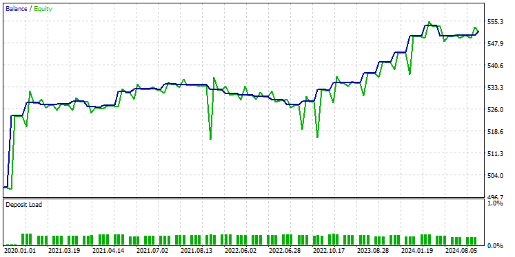
我采用了与以前相同的测试器设置,结果如下。

这次整体交易准确率约为 74%,低于我们之前模型的准确率,但仍然非常出色!
组合卷积神经网络(CNN)和门控循环单元(GRU)
就像 LSTM 一样,GRU 模型也能够理解长期序列信息和数据之间的关系,尽管与 LSTM 模型相比采用了极简的方式。
我们可如其它 RNN 模型一样实现它,我们只在构建 CNN 模型架构的代码中修改模型类型。
from tensorflow.keras.layers import GRU

# Define the CNN model

model = Sequential()
model.add(Conv1D(filters=16,
                 kernel_size=3,
                 activation='relu',
                 strides=2,
                 padding='causal',
                 input_shape=(time_step, X_train.shape[2])
                )
         )

model.add(MaxPooling1D(pool_size=2))


model.add(GRU(50, activation='relu'))
model.add(Dropout(0.5))
model.add(Dense(50, activation='relu'))
model.add(Dropout(0.5))
model.add(Dense(units=len(np.unique(y)), activation='softmax'))  # For binary classification (e.g., buy/sell signal)

model.summary()
模型经过训练和验证后,该模型达成了与 LSTM 相似的准确率,测试数据的准确率为 53%。
7/7 ━━━━━━━━━━━━━━━━━━━━ 1s 41ms/step
Classification Report
               precision    recall  f1-score   support

           0       0.69      0.39      0.50       117
           1       0.45      0.73      0.55        78

    accuracy                           0.53       195
   macro avg       0.57      0.56      0.53       195
weighted avg       0.59      0.53      0.52       195
我们加载 ONNX 格式的 GRU 模型,并将其伸缩器参数加载到二进制文件之中。
#resource "\\Files\\gru+cnn.TSLA.D1.onnx" as uchar onnx_model[]
#resource "\\Files\\gru+cnn.TSLA.D1.standard_scaler_mean.bin" as double standardization_mean[]
#resource "\\Files\\gru+cnn.TSLA.D1.standard_scaler_scale.bin" as double standardization_std[]

#include <MALE5\Convolutional Neural Networks(CNNs)\ConvNet.mqh>
#include <MALE5\preprocessing.mqh>

CConvNet cnn;
StandardizationScaler *scaler;
再次,其余代码与简单 RNN EA 中所用代码相同。
在测试器上采用相同设置测试模型后,结果如下。
GRU 模型提供了大约 61% 的准确率,不如前两个模型优秀,但确实是一个不错的准确率。
后记
卷积神经网络(CNN)与递归神经网络(RNN)的集成可成为预测股票市场的强大方法,为揭示数据中隐藏的形态和时态依赖关系提供了潜力。然而,这种组合相对不常见,并且会带来一定的挑战。主要风险之一是过度拟合,尤其是在将如此复杂的模型应用于相对简单的问题时。过拟合会导致模型在训练数据上表现良好,但无法普适到新数据。
此外,将 CNN 和 RNN 组合在一起的复杂性,会导致巨大的计算成本,特别是如果您决定通过添加更多密集层、或增加神经元数量来扩展模型。必须仔细平衡模型复杂性、与可用资源、和手头的问题。
平安出行。
跟踪机器学习模型的开发,在 GitHub 存储库 上有更多本系列文章的讨论内容。
附件表
文件名 | 文件类型 | 说明/用法 |
|---|---|---|
Experts\CNN + GRU EA.mq5 Experts\CNN + LSTM EA.mq5 Experts\CNN + RNN EA.mq5 | 智能系统 | 加载 ONNX 模型,并在 MetaTrader 5 中测试交易策略的交易机器人。 |
ConvNet.mqh preprocessing.mqh | 包含文件 |
|
Files\ *.onnx | ONNX 模型 | 本文中讨论的 ONNX 格式的机器学习模型 |
| Files\*.bin | 二进制文件 | 加载每个模型的标准化伸缩器参数的二进制文件 |
Jupyter Notebook\cnns-rnns.ipynb | python/Jupyter notebook | 本文中讨论的所有 Python 代码都可在该笔记簿中找到。 |
本文由MetaQuotes Ltd译自英文
原文地址: https://www.mql5.com/en/articles/15585
注意: MetaQuotes Ltd.将保留所有关于这些材料的权利。全部或部分复制或者转载这些材料将被禁止。
本文由网站的一位用户撰写,反映了他们的个人观点。MetaQuotes Ltd 不对所提供信息的准确性负责,也不对因使用所述解决方案、策略或建议而产生的任何后果负责。


 Connexus请求解析(第六部分):创建HTTP请求与响应