数据科学和机器学习（第 28 部分）：使用 AI 预测 EURUSD 的多个期货

MetaTrader 5 — 交易 | 14 四月 2025, 07:58

591

Omega J Msigwa

内容

概述

在运用机器学习进行财经数据分析的世界，目标往往是基于历史数据预测未来值。而预测下一个立即值非常实用，正如我们在本系列的多篇文章中所讨论的那样。在真实世界应用中，有许多状况，其中我们或许需要预测多个未来值，而非一个。预测各种连续值的尝试称为多步或多横向范围预测。

多步预测在各个领域，诸如金融、天气预报、供应链管理、和医疗保健、等等都至关重要。举例，在金融市场中，投资者需要预测未来若干天、数周、甚至数月的股票价格或汇率。在天气预报中，对未来数天或数周的准确预报有助于规划和灾害管理。

本文假设您对机器学习和 AI、ONNX、如何在 MQL5 中使用 ONNX 模型、线性回归、LightGBM、和神经网络都有基本的了解。

多步预测过程涉及若干种方法，其每种都有其强项和弱项。这些方法包括。

直接多步预测
递归多步预测
多输出模型
向量自回归（VAR）（将在下一篇文章中讨论）

在本文中，我们将探讨这些方法，它们的应用，以及如何运用各种机器学习和统计技术来实现它们。通过理解和应用多步预测，我们能够针对 EURUSD 的未来做出更有见地的决策。

# Create target variables for multiple future steps

def create_target(df, future_steps=10):
    target = pd.concat([df['Close'].shift(-i) for i in range(1, future_steps + 1)], axis=1) # using close prices for the next i bar
    target.columns = [f'target_close_{i}' for i in range(1, future_steps + 1)] # naming the columns
    return target

# Combine features and targets

new_df = pd.DataFrame({
    'Open': df['Open'],
    'High': df['High'],
    'Low': df['Low'],
    'Close': df['Close']
})


future_steps = 5

target_columns = create_target(new_df, future_steps).dropna()
combined_df = pd.concat([new_df, target_columns], axis=1) #concatenating the new pandas dataframe with the target columns

combined_df = combined_df.dropna() #droping rows with NaN values caused by shifting values

target_cols_names = [f'target_close_{i}' for i in range(1, future_steps + 1)]

X = combined_df.drop(columns=target_cols_names).values #dropping all target columns from the x array
y = combined_df[target_cols_names].values # creating the target variables

print(f"x={X.shape} y={y.shape}")
combined_df.head(10)

直接多步预测

直接多步预测方法是单独训练的预测模型，为您预测想要的每个未来时间步。例如，如果我们要预测接下来 5 个时间步的值，我们将训练 5 个不同的模型。一个预测第一步，另一个预测第二步，依此类推。

在直接多步预测中，每个模型都设计用于预测特定横向范围。这种方式允许每个模型专注于相应未来时间步有关的特定形态和关系，潜在提升每个预测的准确性。不过，这也意味着您需要训练和维护多个模型，而这肯定是资源密集型的。

我们尝试使用 LightGBM 机器学习模型进行多步预测。

首先，我们创建一个函数来处理来自多步的数据。

准备数据

Python 代码

def multi_steps_data_process(data, step, train_size=0.7, random_state=42):

    # Since we are using the OHLC values only
    
    data["next signal"] = data["Signal"].shift(-step) # The target variable from next n future values
    data = data.dropna()
        
    y = data["next signal"]
    X = data.drop(columns=["Signal", "next signal"])
    
    return train_test_split(X, y, train_size=train_size, random_state=random_state)

该函数创建新的目标变量，对应数据集中的 “Signal” 列。目标变量取自 "signal" 列中步骤索引+1 处的数值。

假设您得到。

信号
1
2
3
4
5

在步骤 1 处，下一个信号将为 2，在步骤 2 中，下一个信号将为 3，依此类推。

这意味着在步 1 处，我们以该方式创建数据集，目标变量是自未来 1 根柱线的值，依此类推。所有自变量都保持不变。

在本文中，我们将采用来自 EURUSD H1、时间帧、1000 根柱线中获取的数据。

Python 代码

df = pd.read_csv("/kaggle/input/eurusd-period-h1/EURUSD.PERIOD_H1.csv")

print(df.shape)
df.head(10)

输出

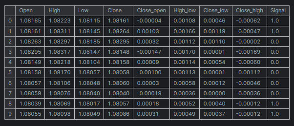
为简单起见，我创建的迷你数据集仅有五（5）个变量。

“Signal” 列代表蜡烛的看涨或看跌信号，它是按逻辑创建的，每当收盘价大于开盘价时，信号被赋值 1，反之赋值 0。

现在我们有一个创建多步数据的函数，我们来声明处理每步的模型。

训练多个模型进行预测

针对每个时间步的模型手动硬编码，肯定既耗时又低效，在循环内编码会更容易、更有效。在循环内，我们执行所有必要的工作，例如训练、验证、和保存模型，以供 MetaTrader 5 外部使用。

Python 代码

for pred_step in range(1, 6): # We want to 5 future values

    lgbm_model = lgbm.LGBMClassifier(**params)
    
    
    X_train, X_test, y_train, y_test = multi_steps_data_process(new_df, pred_step) # preparing data for the current step
    
    
    lgbm_model.fit(X_train, y_train) # training the model for this step
    
    # Testing the trained mdoel 
    
    test_pred = lgbm_model.predict(X_test) # Changes from bst to pipe
 
        
    # Ensuring the lengths are consistent

    if len(y_test) != len(test_pred):
        test_pred = test_pred[:len(y_test)]
        
    
    print(f"model for next_signal[{pred_step} accuracy={accuracy_score(y_test, test_pred)}")
    
    #  Saving the model in ONNX format, Registering ONNX converter

    update_registered_converter(
        lgbm.LGBMClassifier,
        "GBMClassifier",
        calculate_linear_classifier_output_shapes,
        convert_lightgbm,
        options={"nocl": [False], "zipmap": [True, False, "columns"]},
    )
    # Final LightGBM conversion to ONNX

    model_onnx = convert_sklearn(
        lgbm_model,
        "lightgbm_model",
        [("input", FloatTensorType([None, X_train.shape[1]]))],
        target_opset={"": 12, "ai.onnx.ml": 2},
    )

    # And save.
    with open(f"lightgbm.EURUSD.h1.pred_close.step.{pred_step}.onnx", "wb") as f:
        f.write(model_onnx.SerializeToString())

输出

model for next_signal[1 accuracy=0.5033333333333333
model for next_signal[2 accuracy=0.5566666666666666
model for next_signal[3 accuracy=0.4866666666666667
model for next_signal[4 accuracy=0.4816053511705686
model for next_signal[5 accuracy=0.5317725752508361

令人惊讶的是，预测后边第二根柱线的模型是最准确的模型，准确率为 55%，其次是预测后边第五根柱线的模型，其提供的准确率为 53%。

在 MetaTrader 5 中加载模型进行预测

我们首先将所有以 ONNX 格式保存的 LightGBM AI 模型作为资源文件集成到我们的智能系统当中。

MQL5 代码

#resource "\\Files\\lightgbm.EURUSD.h1.pred_close.step.1.onnx" as uchar model_step_1[]
#resource "\\Files\\lightgbm.EURUSD.h1.pred_close.step.2.onnx" as uchar model_step_2[]
#resource "\\Files\\lightgbm.EURUSD.h1.pred_close.step.3.onnx" as uchar model_step_3[]
#resource "\\Files\\lightgbm.EURUSD.h1.pred_close.step.4.onnx" as uchar model_step_4[]
#resource "\\Files\\lightgbm.EURUSD.h1.pred_close.step.5.onnx" as uchar model_step_5[]

#include <MALE5\Gradient Boosted Decision Trees(GBDTs)\LightGBM\LightGBM.mqh>

CLightGBM *light_gbm[5]; //for storing 5 different models
MqlRates rates[];

然后，我们初始化 5 个不同的模型。

MQL5 代码

int OnInit()
  {
//---

   for (int i=0; i<5; i++)
     light_gbm[i] = new CLightGBM(); //Creating LightGBM objects

//---
   
   if (!light_gbm[0].Init(model_step_1))
     {
       Print("Failed to initialize model for step=1 predictions");
       return INIT_FAILED;
     }
   
   if (!light_gbm[1].Init(model_step_2))
     {
       Print("Failed to initialize model for step=2 predictions");
       return INIT_FAILED;
     }
   
   if (!light_gbm[2].Init(model_step_3))
     {
       Print("Failed to initialize model for step=3 predictions");
       return INIT_FAILED;
     }
   
   if (!light_gbm[3].Init(model_step_4))
     {
       Print("Failed to initialize model for step=4 predictions");
       return INIT_FAILED;
     }
   
   if (!light_gbm[4].Init(model_step_5))
     {
       Print("Failed to initialize model for step=5 predictions");
       return INIT_FAILED;
     }
      
   
   return(INIT_SUCCEEDED);
  }

最后，我们可从前一根柱线收集开盘价、最高价、最低价、和收盘价数值，并据它们从所有 5 个不同的模型中获取预测。

MQL5 代码

void OnTick()
  {
//---
   
   CopyRates(Symbol(), PERIOD_H1, 1, 1, rates);
   vector input_x = {rates[0].open, rates[0].high, rates[0].low, rates[0].close};
   
   string comment_string = "";
   int signal = -1;
   
   for (int i=0; i<5; i++)
    {
      signal = (int)light_gbm[i].predict_bin(input_x);
      comment_string += StringFormat("\n Next[%d] bar predicted signal=%s",i+1, signal==1?"Buy":"Sell");
    }
    
   Comment(comment_string);
  }

成果

直接多步预测的强项

每个模型都专门用于特定的预测横向范围，潜在会导致每步的预测更准确。
训练单独的模型能够直截了当，尤其在您采用简单机器学习算法时。
您可为每步选择不同的模型或算法，在处理不同的预测挑战时获得更大的灵活性。

直接多步预测的弱项

它需要训练和维护多个模型，肯定既昂贵又耗时。
不像是递归方法，一步中的误差不会直接传播到下一步，这既是强项也是弱项。这可能会导致步骤之间的不一致。
每个模型都是独立的，或许无法像统一方法那样有效地捕获预测横向范围之间的依赖关系。

递归多步预测

递归多步预测，也称为迭代预测，其是采用一个单一模型进行提前一步预测的方法。然后，该预测将反馈到模型中，以便进行下一次预测。重复该过程，直到对所需的未来时间步数完成预测。

在递归多步预测中，模型经过训练，以便预测下一个立即值。一旦该值预测之后，它会被添加到输入数据当中，并用于预测下一个值。该方法迭代撬动相同的模型。

为达此目的，我们将使用线性回归模型，据前一收盘价来预测下一个收盘价，以这种方式预测的收盘价，能够作为下一次迭代的输入，依此类推。这种方式看似很容易与单个自变量（feature）配合工作。

Python 代码

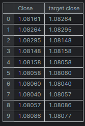
new_df = pd.DataFrame({
    'Close': df['Close'],
    'target close': df['Close'].shift(-1) # next bar closing price
})

然后。

new_df = new_df.dropna() # after shifting we want to drop all NaN values

X = new_df[["Close"]].values # Assigning close values into a 2D x array
y = new_df["target close"].values

print(new_df.shape)
new_df.head(10)

输出

训练 & 测试线性回归模型

在训练模型之前，我们拆分数据且无需随机化。这能够帮助模型捕获数值之间的时态依赖关系，正如我们所知下一个收盘价会受到前一个收盘价的影响。

model = Pipeline([
    ("scaler", StandardScaler()),
    ("linear_regression", LinearRegression())
])


# Split the data into training and test sets

train_size = int(len(new_df) * 0.7)
X_train, X_test = X[:train_size], X[train_size:]
y_train, y_test = y[:train_size], y[train_size:]

# Train the model
model.fit(X_train, y_train)

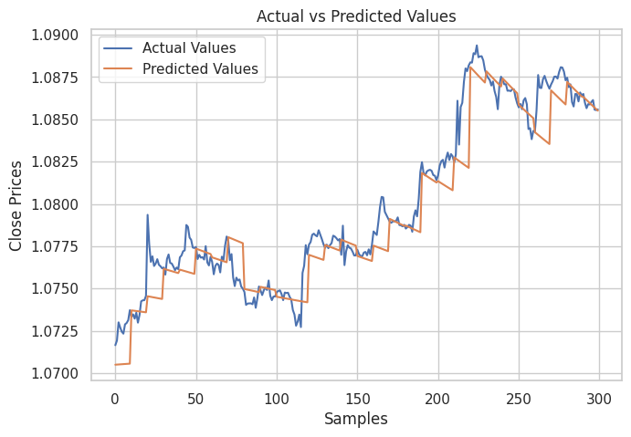
然后，我创建了一个图表来展示测试样本中的实际值及其预测值，是以分析模型在进行预测时的有效性。

# Testing the Model

test_pred = model.predict(X_test) # Make predictions on the test set

# Plot the actual vs predicted values
plt.figure(figsize=(7.5, 5))
plt.plot(y_test, label='Actual Values')
plt.plot(test_pred, label='Predicted Values')
plt.xlabel('Samples')
plt.ylabel('Close Prices')
plt.title('Actual vs Predicted Values')
plt.legend()
plt.show()

成果

从上图可见。该模型做出了不错的预测，它在测试样本上的准确率为 98%，不过，图表中的预测是线性模型依据历史数据集上的性能，以正常方式而非递归格式进行预测。 为了让模型进行递归预测，我们需要为这项工作创建一个自定义函数。

Python 代码

# Function for recursive forecasting
def recursive_forecast(model, initial_value, steps):
    predictions = []
    current_input = np.array([[initial_value]])
    
    for _ in range(steps):
        prediction = model.predict(current_input)[0]
        predictions.append(prediction)
        
        # Update the input for the next prediction
        current_input = np.array([[prediction]])
    
    return predictions

然后，我们就能得到 10 根柱线的未来预测。

current_close = X[-1][0]  # Use the last value in the array

# Number of future steps to forecast
steps = 10

# Forecast future values
forecasted_values = recursive_forecast(model, current_close, steps)

print("Forecasted Values:")
print(forecasted_values)

输出

Forecasted Values:
[1.0854623040804965, 1.0853751608200348, 1.0852885667357617, 1.0852025183667728, 1.0851170122739744, 1.085032045039946, 1.0849476132688034, 1.0848637135860637, 1.0847803426385094, 1.0846974970940555]

为了测试递归模型的准确性，我们可用上面的函数 recursive_forecast，从当前索引处的 10 个时间步之后，循环遍历历史，预测下 10 个时间步。

predicted = []

for i in range(0, X_test.shape[0], steps):
    
    current_close = X_test[i][0]  # Use the last value in the test array
    
    forecasted_values = recursive_forecast(model, current_close, steps)
    predicted.extend(forecasted_values)
    
print(len(predicted))

输出

递归模型准确率为 91%。

最后，我们将线性回归模型保存为 ONNX 格式，其可与 MQL5 兼容。

# Convert the trained pipeline to ONNX
initial_type = [('float_input', FloatTensorType([None, 1]))]
onnx_model = convert_sklearn(model, initial_types=initial_type)

# Save the ONNX model to a file
with open("Lr.EURUSD.h1.pred_close.onnx", "wb") as f:
    f.write(onnx_model.SerializeToString())

print("Model saved to Lr.EURUSD.h1.pred_close.onnx")

在 MQL5 中进行递归预测。

我们从往智能系统中添加线性回归 ONNX 模型开始。

#resource "\\Files\\Lr.EURUSD.h1.pred_close.onnx" as uchar lr_model[]

然后，我们导入线性回归模型处理类。

#include <MALE5\Linear Models\Linear Regression.mqh>
CLinearRegression lr;

在 OnInit 函数内初始化模型之后，我们就能得到前一根已收盘柱线的收盘价，然后预测接下来的 10 根柱线。

int OnInit()
  {
//---
   
   if (!lr.Init(lr_model))
     return INIT_FAILED;
   
//---
   
   ArraySetAsSeries(rates, true);

   return(INIT_SUCCEEDED);
  }
//+------------------------------------------------------------------+
//| Expert tick function                                             |
//+------------------------------------------------------------------+
void OnTick()
  {
//---
   
   CopyRates(Symbol(), PERIOD_H1, 1, 1, rates);
   vector input_x = {rates[0].close}; //get the previous closed bar close price
   
   vector predicted_close(10); //predicted values for the next 10 timestepps
   
   for (int i=0; i<10; i++)
    {
      predicted_close[i] = lr.predict(input_x);
      input_x[0] = predicted_close[i]; //The current predicted value is the next input
    }
   
   Print(predicted_close);
  }

输出

OR      0       16:39:37.018    Recursive-Multi step forecasting (EURUSD,H4)    [1.084011435508728,1.083933353424072,1.083855748176575,1.083778619766235,1.083701968193054,1.083625793457031,1.083550095558167,1.08347487449646,1.083400130271912,1.083325862884521]

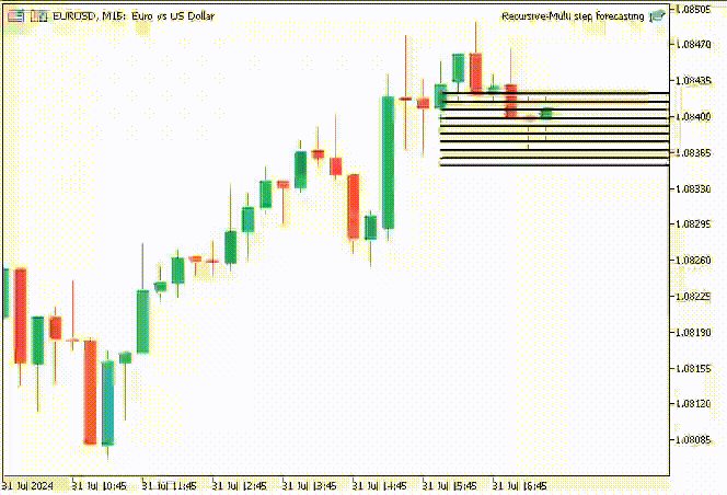
为了让事情更有趣，我决定创建趋势线对象，在主图表上显示 10 个时间步的预测值。

   if (NewBar())
    {
      for (int i=0; i<10; i++)
       {
         predicted_close[i] = lr.predict(input_x);
         input_x[0] = predicted_close[i]; //The current predicted value is the next input
        
        //---
        
            ObjectDelete(0, "step"+string(i+1)+"-prediction"); //delete an object if it exists
            TrendCreate("step"+string(i+1)+"-prediction",rates[0].time, predicted_close[i], rates[0].time+(10*60*60), predicted_close[i], clrBlack); //draw a line starting from the previous candle to 10 hours forward
       }
    }

TrendCreate 函数创建一条较短的水平趋势线，从前一根收盘柱线开始，向前 10 根柱线。

成果

递归多步预测的优势

由于仅训练和维护一个模型，这简化了实现，并降低了计算资源。
由于迭代使用相同的模型，故它在整个预测横向范围内均保持一致性。

递归多步预测的弱项

早期预测中的误差会在后续预测中传播和放大，潜在降低整体准确性。
该方式假设模型捕获的关系在预测横向范围内保持稳定，但情况或许并非总是如此。

使用多输出模型进行多步预测

多输出模型设计用于一次预测多个数值，我们可利用这一优势，让模型同时预测未来时间步。多输出模型具有多个输出，逐一对应一个未来时间步，取代了针对每个预测横向范围训练单独的模型、或递归单个模型。

在多输出模型中，模型经过训练，可在一次通验中生成一个预测向量。这意味着该模型学会直接理解不同未来时间步之间的关系和依赖关系。该方式能用神经网络很好地实现，因其具有产生多个输出的能力。

为多输出神经网络模型准备数据集

我们必须准备目标变量，即我们打算由经训练神经网络模型进行预测的所有时间步。

Python 代码

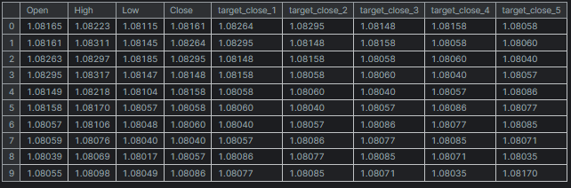
# Create target variables for multiple future steps

def create_target(df, future_steps=10):
    target = pd.concat([df['Close'].shift(-i) for i in range(1, future_steps + 1)], axis=1) # using close prices for the next i bar
    target.columns = [f'target_close_{i}' for i in range(1, future_steps + 1)] # naming the columns
    return target

# Combine features and targets

new_df = pd.DataFrame({
    'Open': df['Open'],
    'High': df['High'],
    'Low': df['Low'],
    'Close': df['Close']
})


future_steps = 5

target_columns = create_target(new_df, future_steps).dropna()
combined_df = pd.concat([new_df, target_columns], axis=1) #concatenating the new pandas dataframe with the target columns

combined_df = combined_df.dropna() #droping rows with NaN values caused by shifting values

target_cols_names = [f'target_close_{i}' for i in range(1, future_steps + 1)]

X = combined_df.drop(columns=target_cols_names).values #dropping all target columns from the x array
y = combined_df[target_cols_names].values # creating the target variables

print(f"x={X.shape} y={y.shape}")
combined_df.head(10)

输出

x=(995, 4) y=(995, 5)

训练和测试多输出神经网络

我们从定义一个顺序神经网络模型开始。

Python 代码

# Defining the neural network model
model = Sequential([
    Input(shape=(X.shape[1],)),
    Dense(units = 256, activation='relu'),
    Dense(units = 128, activation='relu'),
    Dense(units = future_steps)
])

# Compiling the model
adam = Adam(learning_rate=0.01)
model.compile(optimizer=adam, loss='mse')

# Mmodel summary
model.summary()

输出

┏━━━━━━━━━━━━━━━━━━━━━━━━━━━━━━━━━┳━━━━━━━━━━━━━━━━━━━━━━━━┳━━━━━━━━━━━━━━━┓
┃ Layer (type)                    ┃ Output Shape           ┃       Param # ┃
┡━━━━━━━━━━━━━━━━━━━━━━━━━━━━━━━━━╇━━━━━━━━━━━━━━━━━━━━━━━━╇━━━━━━━━━━━━━━━┩
│ dense (Dense)                   │ (None, 256)            │         1,280 │
├─────────────────────────────────┼────────────────────────┼───────────────┤
│ dense_1 (Dense)                 │ (None, 128)            │        32,896 │
├─────────────────────────────────┼────────────────────────┼───────────────┤
│ dense_2 (Dense)                 │ (None, 5)              │           645 │
└─────────────────────────────────┴────────────────────────┴───────────────┘
 Total params: 34,821 (136.02 KB)
 Trainable params: 34,821 (136.02 KB)
 Non-trainable params: 0 (0.00 B)

然后，我们将数据分别切分为训练样本和测试样本，这与我们在递归多步预测中的行事不同。这次，我们用 42 个随机种子把数据随机化之后，再对数据进行拆分，鉴于我们不想让模型理解顺序形态，正如我们相信神经网络理解这些数据中的非线性关系方面会表现得更好。

最后，我们采用训练数据训练神经网络模型。

# Split the data into training and test sets
X_train, X_test, y_train, y_test = train_test_split(X, y, train_size=0.7, random_state=42)

scaler = MinMaxScaler()

X_train = scaler.fit_transform(X_train)
X_test = scaler.transform(X_test)

# Training the model

early_stopping = EarlyStopping(monitor='val_loss', patience=5, restore_best_weights=True) # stop training when 5 epochs doesn't improve

history = model.fit(X_train, y_train, epochs=20, validation_split=0.2, batch_size=32, callbacks=[early_stopping])

据测试数据集测试模型之后。

# Testing the Model

test_pred = model.predict(X_test) # Make predictions on the test set

# Plotting the actual vs predicted values for each future step
plt.figure(figsize=(7.5, 10))
for i in range(future_steps):
    plt.subplot((future_steps + 1) // 2, 2, i + 1)  # subplots grid 
    plt.plot(y_test[:, i], label='Actual Values')
    plt.plot(test_pred[:, i], label='Predicted Values')
    plt.xlabel('Samples')
    plt.ylabel(f'Close Price +{i+1}')
    plt.title(f'Actual vs Predicted Values (Step {i+1})')
    plt.legend()

plt.tight_layout()
plt.show()

# Evaluating the model for each future step
for i in range(future_steps):
    accuracy = r2_score(y_test[:, i], test_pred[:, i])
    print(f"Step {i+1} - R^2 Score: {accuracy}")

下面是成果

Step 1 - R^2 Score: 0.8664635514027637
Step 2 - R^2 Score: 0.9375671150885528
Step 3 - R^2 Score: 0.9040736780305894
Step 4 - R^2 Score: 0.8491904738263638
Step 5 - R^2 Score: 0.8458062142647863

神经网络针对这个回归问题产生的结果令人印象深刻。下面的代码展示出如何在 Python 中获取预测。

# Predicting multiple future values

current_input = X_test[0].reshape(1, -1) # use the first row of the test set, reshape the data also
predicted_values = model.predict(current_input)[0] # adding[0] ensures we get a 1D array instead of 2D

print("Predicted Future Values:")
print(predicted_values)

输出

1/1 ━━━━━━━━━━━━━━━━━━━━ 0s 21ms/step
Predicted Future Values:
[1.0892788 1.0895394 1.0892794 1.0883198 1.0884078]

然后我们就能将该神经网络模型保存为 ONNX 格式，并将定标器文件保存为二进制格式文件。

import tf2onnx

# Convert the Keras model to ONNX
spec = (tf.TensorSpec((None, X_train.shape[1]), tf.float16, name="input"),)
model.output_names=['output']

onnx_model, _ = tf2onnx.convert.from_keras(model, input_signature=spec, opset=13)

# Save the ONNX model to a file
with open("NN.EURUSD.h1.onnx", "wb") as f:
    f.write(onnx_model.SerializeToString())
    
# Save the used scaler parameters to binary files

scaler.data_min_.tofile("NN.EURUSD.h1.min_max.min.bin")
scaler.data_max_.tofile("NN.EURUSD.h1.min_max.max.bin")

最后，我们就能在 MQL5 中使用保存的模型、及其数据定标器参数。

在 MQL5 中获取神经网络多步预测

我们从往智能系统里添加模型、和最小-最大定标器参数开始。

#resource "\\Files\\NN.EURUSD.h1.onnx" as uchar onnx_model[]; //rnn model in onnx format
#resource "\\Files\\NN.EURUSD.h1.min_max.max.bin" as double min_max_max[];
#resource "\\Files\\NN.EURUSD.h1.min_max.min.bin" as double min_max_min[];

然后，我们导入回归神经网络 ONNX 类，意即 MinMax 定标器函数库处理程序。

#include <MALE5\Neural Networks\Regressor Neural Nets.mqh>
#include <MALE5\preprocessing.mqh>

CNeuralNets nn;
MinMaxScaler *scaler;

之后，我们就能初始化神经网络模型和定标器，并从模型中得到最终预测。

MqlRates rates[];
//+------------------------------------------------------------------+
//| Expert initialization function                                   |
//+------------------------------------------------------------------+
int OnInit()
  {
//---

   if (!nn.Init(onnx_model))
     return INIT_FAILED;
   
   scaler = new MinMaxScaler(min_max_min, min_max_max); //Initializing the scaler, populating it with trained values
   
//---
   
   ArraySetAsSeries(rates, true);
   
   return(INIT_SUCCEEDED);
  }
//+------------------------------------------------------------------+
//| Expert deinitialization function                                 |
//+------------------------------------------------------------------+
void OnDeinit(const int reason)
  {
//---
     if (CheckPointer(scaler)!=POINTER_INVALID)
       delete (scaler);
  }
//+------------------------------------------------------------------+
//| Expert tick function                                             |
//+------------------------------------------------------------------+
void OnTick()
  {
//---

   CopyRates(Symbol(), PERIOD_H1, 1, 1, rates);
   vector input_x = {rates[0].open, rates[0].high, rates[0].low, rates[0].close};
   input_x = scaler.transform(input_x); // We normalize the input data
   
   vector preds = nn.predict(input_x);
   
   Print("predictions = ",preds);
  }

输出

2024.07.31 19:13:20.785 Multi-step forecasting using Multi-outputs model (EURUSD,H4)    predictions = [1.080284595489502,1.082370758056641,1.083482265472412,1.081504583358765,1.079929828643799]

为了让事情更有趣，我在图表上添加趋势线来标记所有神经网络的未来预测。

void OnTick()
  {
//---

   CopyRates(Symbol(), PERIOD_H1, 1, 1, rates);
   vector input_x = {rates[0].open, rates[0].high, rates[0].low, rates[0].close};
   
   if (NewBar())
    {
      input_x = scaler.transform(input_x); // We normalize the input data 
      vector preds = nn.predict(input_x);
      
      for (int i=0; i<(int)preds.Size(); i++)
       {  
        //---
        
            ObjectDelete(0, "step"+string(i+1)+"-prediction"); //delete an object if it exists
            TrendCreate("step"+string(i+1)+"-prediction",rates[0].time, preds[i], rates[0].time+(5*60*60), preds[i], clrBlack); //draw a line starting from the previous candle to 5 hours forward
       }
    }
  }

这次，我们得到的预测线比用递归线性回归模型获得的预测线更好看。

使用多输出模型进行多步预测概览

优势

通过一次性预测多步，该模型可以捕获未来时间步之间的关系和依赖关系。
仅需一个模型，这简化了实现和维护。
该模型学习在整个预测横向范围内生成一致的预测。

缺点

训练一个模型来输出多个未来值肯定更复杂，且或许需要更复杂的架构，尤其对于神经网络。
根据模型的复杂度，它或许需要更多的计算资源，以便训练和推理。
存在过度拟合的风险，尤其是在预测横向范围很长，且模型过于专对训练数据。

在交易策略中利用多步预测

多步预测，尤其是用神经网络和 LightGBM 等模型，可启用基于预测的市场走势进行动态调整，据此显著强化各种交易策略。在网格交易中，多步预测允许动态入场，而非设置固定订单，根据预期的价格变化进行调整，从而提升系统对市场条件的响应能力。

对冲策略也从中受益，因为预测提供了关于何时开仓、或平仓，以防止潜在亏损的指导，譬如在预测到下跌趋势时做空、或购入看跌期权。甚至，在趋势检测中，经由预测来理解未来的市场方向，有助于交易者相应地校准他们的策略，要么偏重空仓，要么多仓离场，从而避免亏损。

最后，在高频交易（HFT）中，快速多步预测可以指导算法利用短期价格走势，基于即将来临的几秒钟、或几分钟内预测的价格变化，及时执行买卖订单，从而提高盈利能力。

底线

在金融分析和外汇交易中，如本文前一章节所述，能够预测多个未来值非常实用。本篇旨在为您提供如何应对这一挑战的不同方式。在下一篇文章中，我们将探讨向量自回归，这是一种为分析多个值的任务而构建的技术，也可预测多个值。

平安出行。

跟踪机器学习模型的开发，在 GitHub 存储库上有更多本系列文章的讨论内容。

附件表

文件名	文件类型	说明 & 用法
Direct Muilti step Forecasting.mq5 Multi-step forecasting using multi-outputs model.mq5 Recursive-Multi step forecasting.mq5	智能系统	该 EA 含有使用多个 LightGBM 模型进行多步预测的代码。该 EA 含有利用多输出结构预测多步的神经网络模型。该 EA 含有线性回归迭代预测未来时间步。
LightGBM.mqh	MQL5 函数库文件	含有以 ONNX 格式加载 LightGBM 模型，并用其进行预测的代码。
Linear Regression.mqh	MQL5 函数库文件	含有以 ONNX 格式加载线性回归模型，并用其进行预测的代码。
preprocessing.mqh	MQL5 函数库文件	此文件由 MInMax 定标器组成，这是一种用于归一化输入数据的定标技术。
Regressor Neural Nets.mqh	MQL5 函数库文件	含有加载和部署 ONNX 格式神经网络模型到 MQL5 的代码。
lightgbm.EURUSD.h1.pred_close.step.1.onnx lightgbm.EURUSD.h1.pred_close.step.2.onnx lightgbm.EURUSD.h1.pred_close.step.3.onnx lightgbm.EURUSD.h1.pred_close.step.4.onnx lightgbm.EURUSD.h1.pred_close.step.5.onnx Lr.EURUSD.h1.pred_close.onnx NN.EURUSD.h1.onnx	ONNX 格式的 AI 模型	预测下一步值的 LightGBM 模型 ONNX 格式的简单线性回归模型 ONNX 格式的前馈神经网络
NN.EURUSD.h1.min_max.max.bin NN.EURUSD.h1.min_max.min.bin	二进制文件	分别包含 MIn-max 定标器的最大值和最小值
predicting-multiple-future-tutorials.ipynb	Jupyter 笔记簿	本文中展示的所有 python 代码都位于此文件当中

本文由MetaQuotes Ltd译自英文
原文地址： https://www.mql5.com/en/articles/15465

附加的文件 |

下载ZIP

Attachments.zip (519.77 KB)

注意: MetaQuotes Ltd.将保留所有关于这些材料的权利。全部或部分复制或者转载这些材料将被禁止。

该作者的其他文章

前往讨论

将您自己的 LLM 集成到 EA 中（第 4 部分）：使用 GPU 训练自己的 LLM

随着当今人工智能的快速发展，语言模型（LLMs）是人工智能的重要组成部分，因此我们应该考虑如何将强大的 LLMs 整合到我们的算法交易中。对于大多数人来说，很难根据他们的需求微调这些强大的模型，在本地部署它们，然后将它们应用于算法交易。本系列文章将采取循序渐进的方法来实现这一目标。

在MQL5中实现基于抛物线转向指标（Parabolic SAR）和简单移动平均线（SMA）的快速交易策略算法

在本文中，我们将在MQL5中开发一个快速交易EA，利用抛物线SAR和简单移动平均线（SMA）指标来创建一个响应迅速的交易策略。我们详细介绍了该策略的实施过程，包括指标的使用、信号的生成以及测试和优化过程。

禁忌搜索（TS）

本文讨论了禁忌搜索（Tabu Search）算法，这是一种最早且最为人所知的元启发式方法之一。我们将详细探讨该算法的运行过程，从选择初始解并探索邻近选项开始，重点介绍使用禁忌表。文章涵盖了该算法的关键方面及其特性。

纳什博弈论与隐马尔可夫滤模型在交易中的应用

这篇文章深入探讨了约翰·纳什的博弈论，特别是纳什均衡，在交易中的应用。文章讨论了交易者如何利用Python脚本和MetaTrader 5，依据纳什的原则来识别并利用市场的无效性。文章还提供了实施这些策略的逐步指南，包括使用隐马尔可夫模型（HMM）和统计分析，以提升交易表现。