

Entropy-Based Market Efficiency Indicator in MQL5: Measuring Randomness in Price Returns Using Approximate Entropy
 1 301
1 301
 0
0

Introduction
Trend-following and breakout Expert Advisors treat every market the same: they apply the same crossovers, breakouts, or channel rules whether the return series currently exhibits exploitable serial structure or is effectively a random walk. When returns are structured, those directional rules can have a real statistical edge. When returns are near-random, every signal is noise, and the EA simply pays spreads and commissions on many unprofitable trades — a slow, steady drain that looks like “the strategy isn’t working” but is in fact a regime problem.
MQL5's built-in indicators report price level, momentum, volatility or volume, but none provide a direct, quantitative measure of how predictable the recent return sequence is. Traders therefore rely on eyeballing “chop vs trend” or on volatility proxies that conflate quiet with predictability and volatility with structure — a misleading shortcut, because a series can be volatile yet highly structured (large trending bars) or quiet yet essentially random (tight consolidation with no serial dependence).
This article fills that gap by introducing Approximate Entropy (ApEn) as a practical, native MQL5 tool to measure short-term predictability of closed-bar log-returns. It derives ApEn from first principles, implements a standalone CApEnCalculator class with no external dependencies, supplies a complete subwindow indicator (ApEnIndicator.mq5) that color-codes three regime zones with configurable thresholds, and includes a TestApEn script to verify behavior on synthetic series. Crucially, the article frames ApEn as a gating filter for directional logic (not as a trade signal): read the indicator from your EA via iCustom/CopyBuffer (use shift=1 to avoid intrabar look-ahead), and disable directional entries when ApEn exceeds your chosen upper threshold. The code and inputs are transparent and portable so you can validate and tune the gate for your symbol, timeframe, and execution costs before deploying it live.
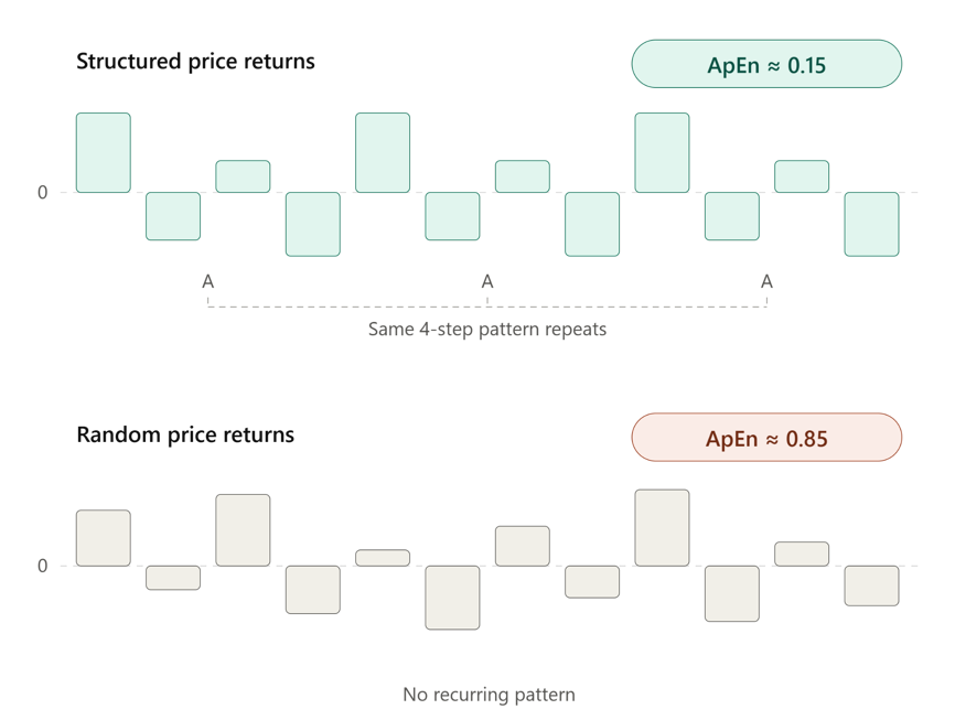
A structured return series (top) repeats the same four-step pattern three times, so knowing one occurrence predicts the next — Approximate Entropy is low. A random return series (bottom) has no recurring structure, so recent history gives no advantage in predicting the next value — Approximate Entropy is high. This is the distinction the indicator built in this article measures directly from price data
Section 1: Market Efficiency and the Predictability Spectrum
The weak-form efficient market hypothesis (EMH) states that current prices fully reflect all information contained in past prices, with the consequence that price changes are serially uncorrelated and unpredictable from price history alone. Under strict weak-form efficiency, no amount of technical analysis applied to past prices should generate excess risk-adjusted returns, because any pattern in past returns would already have been arbitraged away.
Real markets are not uniformly efficient at every moment. Empirical work on market microstructure and on the adaptive market hypothesis suggests that markets cycle between periods of relatively higher predictability — sustained trends, momentum phases, mean-reverting ranges with detectable periodicity — and periods of relatively higher efficiency, where price action resembles a random walk closely enough that no simple technical rule has a durable edge. Trending phases driven by persistent order flow imbalance, and mean-reverting phases driven by a stable equilibrium price with noise around it, both leave a statistical signature: knowing the recent path of prices narrows the distribution of the next move. Consolidation phases and the period immediately following a news shock, by contrast, often display close to maximal unpredictability — the recent path provides little to no information about the next tick.
A static indicator — a fixed-period moving average, a fixed-period RSI — cannot distinguish these two regimes because it does not measure predictability at all; it measures level, momentum, or dispersion. Two series with identical volatility and identical drift can have completely different entropy: one might be a smooth sine wave with noise, the other a sequence of independent draws with the same variance. A complexity measure that operates directly on the information content of the return sequence, recomputed adaptively over a rolling window, is needed to make this distinction explicit and quantitative rather than left to visual judgment. Approximate Entropy is one such measure, and it is the subject of the remainder of this article.
Section 2: The Mathematics of Approximate Entropy
Entropy and predictability
A time series is said to have low entropy when it contains repeating structural patterns — sequences of values that recur, or that are followed by similar continuations each time they occur. In a low-entropy series, knowing the most recent few observations provides real information about what comes next: the conditional distribution of the next value, given recent history, is narrower than the unconditional distribution. A time series is said to have high entropy when it is close to maximally unpredictable — the conditional distribution of the next value given recent history is approximately the same as the unconditional distribution, meaning recent history confers no forecasting advantage.
This is exactly the language in which weak-form market efficiency is framed: an efficient series is one in which past prices give no edge in forecasting future prices. Low ApEn therefore corresponds to a market that is, in the entropy sense, behaving inefficiently — exhibiting exploitable serial structure — while high ApEn corresponds to a market behaving efficiently, in the weak-form sense, over the window measured.
Template vectors
Given a time series of returns u(1), u(2), ..., u(N), ApEn works by embedding the series into vectors of length m, called template vectors:
x_m(i) = [u(i), u(i+1), ..., u(i+m-1)] for i = 1, ..., N-m+1
Each template vector x_m(i) is simply a contiguous subsequence of m consecutive returns, starting at position i. There are N - m + 1 such vectors for a given m, since the last valid starting position is N - m + 1 — beyond that point there are not enough remaining observations to fill out a length-m window. The embedding dimension m controls how much recent history is treated as the "pattern" being matched; the algorithm asks, for each template, how many other templates elsewhere in the series look similar to it.
The Chebyshev distance
Similarity between two template vectors is measured using the Chebyshev, or L∞, distance:
d[x_m(i), x_m(j)] = max_{k=0,...,m-1} |u(i+k) - u(j+k)| This takes the maximum absolute difference across all m corresponding components of the two vectors, rather than, say, the sum of squared differences used by Euclidean distance. The Chebyshev distance is chosen for two reasons. First, it is computationally cheaper — it requires only m subtractions, absolute values, and a running maximum, with no squaring or square root. Second, and more importantly for fidelity to the original method, it is the distance used in Pincus's and in Richman and Moorman's original formulations of ApEn and SampEn; using a different metric would not reproduce the statistic these papers, and the broader literature built on them, refer to as "Approximate Entropy."
The C_i^m(r) statistic
For a given tolerance r, define:
C_i^m(r) = (number of j such that d[x_m(i), x_m(j)] <= r) / (N - m + 1) This is the fraction, among all N - m + 1 template vectors of length m in the series, that lie within distance r of the template starting at position i. The count deliberately includes the self-match j = i, since d[x_m(i), x_m(i)] = 0 <= r always holds; this self-match guarantees C_i^m(r) is never zero, which keeps the next step, a logarithm, well-defined. Intuitively, C_i^m(r) measures how common the local pattern around position i is elsewhere in the series — a high value means the pattern recurs often within tolerance r, a low value means it is comparatively unique.
The Phi(m) function
The Phi function averages the log of these per-template match fractions across all starting positions:
Phi^m(r) = (1 / (N - m + 1)) * sum_{i=1}^{N-m+1} ln(C_i^m(r))
Phi^m(r) is a single number summarizing, on average, how predictable length-m patterns are within the series at tolerance r. A series full of recurring length-m patterns produces high C_i^m(r) values for most i, and therefore a Phi^m(r) close to zero (since ln(1) = 0); a series with mostly unique length-m patterns produces low C_i^m(r) values and a more negative Phi^m(r).
The ApEn formula
ApEn is defined as the difference between the Phi function computed at embedding dimension m and at m+1:
ApEn(m, r, N) = Phi^m(r) - Phi^{m+1}(r) The interpretation follows directly from what each term measures: Phi^m(r) summarizes how often length-m patterns recur, and Phi^{m+1}(r) summarizes how often those same patterns, extended by one additional observation, still recur. The difference captures how much extra information that one additional observation carries — equivalently, how much more predictable a length-(m+1) sequence is than a length-m sequence, given the same tolerance.
A low ApEn means that extending a known pattern by one more observation barely reduces its match count: the series is highly self-similar, and knowing m consecutive values gives strong predictive power about the (m+1)-th. A high ApEn means that extending the pattern sharply reduces the match count: knowing m consecutive values provides almost no advantage in predicting the next one, which is the hallmark of near-random behavior.
The tolerance parameter r
The tolerance r determines how strict the matching criterion is. Since absolute price-return magnitudes vary enormously across instruments and across volatility regimes for the same instrument, r is conventionally expressed as a fraction of the standard deviation of the series being analyzed:
r = k * SD(u)
with k commonly chosen between 0.1 and 0.25, and 0.2 the most frequently cited default in the physiological-signal literature where ApEn originated. Scaling r by SD normalizes the tolerance relative to the series' own dispersion, which is what makes ApEn values roughly comparable across instruments with different volatility levels and across different rolling windows of the same instrument as its volatility regime changes over time. The implementation in this article computes SD adaptively from the contents of the current rolling window on every bar, rather than using a single fixed r value computed once — this keeps the tolerance appropriately scaled even as the instrument moves between quiet and volatile periods.
Computational complexity
Computing C_i^m(r) for every i requires comparing every template vector against every other template vector — an all-pairs comparison — which costs O(N²) distance evaluations for a window of N returns, and this must be repeated for both m and m+1.
The practical implication is a direct trade-off between statistical reliability and computational cost: a larger window N gives a more reliable ApEn estimate (since C_i^m(r) is itself an empirical fraction subject to sampling noise at small N), but increases the number of per-bar pairwise comparisons quadratically. A common minimum-sample guideline is N >= 10^m, which for the standard choice m = 2 implies N should be at least 100. The implementation presented here is designed to operate efficiently in the 50-to-200-bar range, which keeps per-bar computation in the low tens of thousands of comparisons — well within what a single indicator recalculation can perform on a closed bar without introducing perceptible delay in MetaTrader 5.
Regime classification thresholds
For financial return series, empirically observed ApEn values typically fall between 0 and approximately 2.0. As a working classification, values below roughly 0.5 are associated with strongly structured behavior — return sequences with substantial detectable serial pattern; values between roughly 0.5 and 1.2 represent a mixed or transitional regime; and values above roughly 1.2 are associated with near-random behavior, where the additional observation in the m+1 embedding adds essentially no predictive information over the m embedding. These thresholds are empirical generalizations, not theoretical constants — they depend on the instrument, the timeframe, and the choice of m and r — and the indicator built in this article exposes both threshold values as configurable inputs rather than hardcoding them.
Section 3: Parameter Selection and Practical Constraints
Before the implementation, the choice of m, r, and N deserves detailed discussion, since each carries a direct, measurable consequence for the indicator's behavior. The embedding dimension m = 2 is the standard choice for financial return series: m = 1 is too coarse, since it only measures whether individual return magnitudes recur rather than any sequential structure, while m = 3 requires N ≥ 1000 for reliable estimates, an impractical sample size for a rolling-window indicator meant to react to changing regimes within a reasonable number of bars. The tolerance factor r = 0.2 · SD is the most common choice in the literature, and the implementation computes SD adaptively from the contents of the rolling window itself, so the tolerance stays correctly scaled to the instrument's current volatility rather than depending on a static estimate computed once at startup.
The O(N²) cost of the all-pairs template comparison has a direct implication for window size. A window of 100 bars requires on the order of 10,000 template comparisons per bar; at 200 bars this grows to roughly 40,000. This is the basis for the recommended operating range of 50 to 200 bars, and it is also the basis for a genuine trade-off the indicator's InpWindowSize input exposes directly to the operator rather than hiding behind a fixed constant.
That trade-off is visible directly by comparing the same instrument under two window settings. Running the indicator on EURUSD H1 with InpWindowSize=100 requires 102 bars of history before the first ApEn value is plotted, since the calculator withholds output until the rolling window is completely full; on a chart with limited available history, this can leave the oscillator blank for a visible stretch at the left edge of the chart. Reducing InpWindowSize to 50 halves that warm-up requirement to 52 bars, and the plotted line begins correspondingly earlier — a direct, observable consequence of the sample-size guideline discussed above, not a change in the underlying algorithm.
The trade-off is that a 50-bar window sits below the N ≥ 10^m = 100 guideline for m = 2, so its ApEn estimates should be treated as more provisional: individual C_i^m(r) fractions are computed over fewer templates, making them more sensitive to the specific return values that happen to occupy the smaller window at any given moment. A shorter window is a reasonable choice for faster visual feedback during testing or for instruments with limited available history, but the 100-bar-or-larger default remains the better choice for live use, where estimate stability is more valuable than a shorter warm-up period.
Section 4: Implementation — ApEnCalculator.mqh
The CApEnCalculator class is the computational core of this article. Its sole responsibility is maintaining a rolling window of return values and computing ApEn over that window on demand; it has no knowledge of bars, prices, or the indicator buffer system, and no dependency on any MQL5 indicator-specific API. This separation means the same class can be instantiated inside a custom indicator, an Expert Advisor, or a script, with no modification, which is the reason it is built as a standalone include file rather than embedded directly in the indicator source.
//+------------------------------------------------------------------+
//|                                             ApEnCalculator.mqh   |
//+------------------------------------------------------------------+
#ifndef APENCALCULATOR_MQH
#define APENCALCULATOR_MQH
//+------------------------------------------------------------------+
//| Class CApEnCalculator                                            |
//| Computes Approximate Entropy over a rolling window of returns    |
//+------------------------------------------------------------------+
class CApEnCalculator
  {
private:
   int               m_m;
   double            m_r_factor;
   double            m_window[];
   int               m_window_size;
   int               m_capacity;
   double            ComputePhi(const double &series[],int n,int m,double r);
   double            ComputeSD(const double &series[],int n);
public:
                     CApEnCalculator(void);
                    ~CApEnCalculator(void);
   bool              Init(int capacity,int m,double r_factor);
   void              Push(double value);
   double            Compute(void);
   bool              IsReady(void);
   void              Reset(void);
  };
The class declares two private helper methods, ComputePhi() and ComputeSD(), which implement the inner mathematics described in Section 2 and are not part of the public interface because callers never need to invoke them directly. The private member m_m stores the embedding dimension, m_r_factor stores the multiplier applied to the window's standard deviation to obtain the tolerance r, m_window[] is the dynamically sized array holding the rolling set of return values, m_window_size tracks how many of the array's slots currently hold valid data (which starts at zero and grows to m_capacity during the warm-up period), and m_capacity is the fixed maximum size of the window, set once in Init().
The public interface consists of Init() to configure and allocate the calculator, Push() to feed one new return value into the rolling window, Compute() to run the full ApEn calculation over the current window contents, IsReady() to query whether the window has reached full capacity, and Reset() to clear all stored state, which is used when the indicator's prev_calculated value resets to zero, as happens on a full chart recalculation.
Constructor
//+------------------------------------------------------------------+
//| Constructor                                                      |
//+------------------------------------------------------------------+
CApEnCalculator::CApEnCalculator(void)
  {
   m_m=2;
   m_r_factor=0.2;
   m_window_size=0;
   m_capacity=0;
  }
The constructor establishes safe default values before Init() is ever called: an embedding dimension of 2, the conventional r factor of 0.2, and a window size and capacity of zero, which leaves the calculator in a state where IsReady() correctly reports false and Compute() correctly returns EMPTY_VALUE until Init() has been explicitly invoked by the caller.
Destructor
//+------------------------------------------------------------------+
//| Destructor                                                       |
//+------------------------------------------------------------------+
CApEnCalculator::~CApEnCalculator(void)
  {
   ArrayFree(m_window);
  }
The destructor releases the dynamic memory held by m_window[] using ArrayFree(). This is declared and defined explicitly, with a non-empty body, in keeping with the requirement that resource-holding classes never rely on an implicit or omitted destructor, even though m_window[] would eventually be reclaimed by the runtime in any case; explicit cleanup keeps the class's resource lifecycle visible and self-documenting.
Init()
//+------------------------------------------------------------------+
//| Init                                                             |
//+------------------------------------------------------------------+
bool CApEnCalculator::Init(int capacity,int m,double r_factor)
  {
   if(capacity<=2 || m<1 || r_factor<=0.0)
      return(false);
   m_capacity=capacity;
   m_m=m;
   m_r_factor=r_factor;
   m_window_size=0;
   if(ArrayResize(m_window,m_capacity)!=m_capacity)
      return(false);
   ArrayInitialize(m_window,0.0);
   return(true);
  }
Init() validates its three arguments before doing any allocation: the capacity must be at least 3 (a window of 2 or fewer cannot support even the m+1 = 3 embedding required internally), the embedding dimension must be at least 1, and the r factor must be strictly positive, since a non-positive tolerance would make every Chebyshev-distance comparison fail except self-matches. If validation passes, the method stores the three configuration values, resets m_window_size to zero to begin a fresh warm-up period, and calls ArrayResize() to allocate the window array to the requested capacity, checking the return value to confirm the resize succeeded before proceeding. ArrayInitialize() then zeroes the newly allocated array so that any stale memory content cannot influence subsequent computation before real data has been pushed into every slot.
Push()
//+------------------------------------------------------------------+
//| Push                                                             |
//+------------------------------------------------------------------+
void CApEnCalculator::Push(double value)
  {
   if(m_capacity<=0)
      return;
   if(m_window_size<m_capacity)
     {
      m_window[m_window_size]=value;
      m_window_size++;
     }
   else
     {
      for(int i=0;i<m_capacity-1;i++)
         m_window[i]=m_window[i+1];
      m_window[m_capacity-1]=value;
     }
  }
Push() implements the rolling-window update. It first guards against being called before Init() has set a valid capacity. While the window has not yet reached m_capacity, the new value is simply appended at the next free slot and m_window_size is incremented, which is the warm-up phase during which Compute() will return EMPTY_VALUE. Once the window is full, each call to Push() shifts every existing element one position toward the start of the array, discarding the oldest value, and writes the new value into the now-vacated final slot, implementing a first-in-first-out rolling buffer of fixed size m_capacity. The shift is O(capacity) per call, which is negligible relative to the O(capacity²) cost of Compute() itself, so it does not change the indicator's overall complexity profile.
ComputeSD()
//+------------------------------------------------------------------+
//| ComputeSD                                                        |
//+------------------------------------------------------------------+
double CApEnCalculator::ComputeSD(const double &series[],int n)
  {
   if(n<=1)
      return(0.0);
   double mean=0.0;
   for(int i=0;i<n;i++)
      mean+=series[i];
   mean/=n;
   double sum_sq=0.0;
   for(int i=0;i<n;i++)
      sum_sq+=(series[i]-mean)*(series[i]-mean);
   return(::MathSqrt(sum_sq/(n-1)));
  }
ComputeSD() computes the sample standard deviation of the supplied series using the conventional two-pass formula: the first loop accumulates the mean, and the second loop accumulates the sum of squared deviations from that mean, which is then divided by n-1 (the sample, rather than population, variance) and passed through MathSqrt(). The :: scope-resolution prefix on MathSqrt() ensures the call resolves to the global MQL5 standard library function rather than to any same-named method that might exist on this class or a derived class. This standard deviation is the basis for the adaptive tolerance r described in Section 2, and is recomputed from the actual window contents each time Compute() runs, so it always reflects current market volatility rather than a stale or externally supplied estimate.
ComputePhi()
//+------------------------------------------------------------------+
//| ComputePhi                                                       |
//+------------------------------------------------------------------+
double CApEnCalculator::ComputePhi(const double &series[],int n,int m,double r)
  {
   int count=n-m+1;
   if(count<=0)
      return(0.0);
   double phi_sum=0.0;
   for(int i=0;i<count;i++)
     {
      int matches=0;
      for(int j=0;j<count;j++)
        {
         double dist=0.0;
         for(int k=0;k<m;k++)
           {
            double diff=::MathAbs(series[i+k]-series[j+k]);
            if(diff>dist)
               dist=diff;
           }
         if(dist<=r)
            matches++;
        }
      double c_i=(double)matches/(double)count;
      phi_sum+=::MathLog(c_i);
     }
   return(phi_sum/count);
  }
ComputePhi() is the direct implementation of the Phi^m(r) function defined in Section 2. The outer index i ranges over every valid template starting position, of which there are count = n - m + 1. For each i, the inner index j ranges over the same set of starting positions, and the innermost loop over k computes the Chebyshev distance between template i and template j by tracking the maximum absolute component-wise difference, using MathAbs(). Whenever that distance is within tolerance r, matches is incremented; because j ranges over all valid positions including j = i, the self-match is automatically counted, matching the definition of C_i^m(r) given earlier. After the inner loops complete, c_i is the fraction of templates matching template i, and its natural logarithm via MathLog() is accumulated into phi_sum. The method returns the average of these log-match-fractions across all count templates, which is exactly Phi^m(r) as defined mathematically.
This method is called twice by Compute(), once with m and once with m+1, and its triple-nested loop structure is the source of the O(N²) per-call cost discussed in Section 3.
Compute()
//+------------------------------------------------------------------+
//| Compute                                                          |
//+------------------------------------------------------------------+
double CApEnCalculator::Compute(void)
  {
   if(m_window_size<m_capacity)
      return(EMPTY_VALUE);
   if(m_capacity<m_m+2)
      return(EMPTY_VALUE);
   double sd=ComputeSD(m_window,m_window_size);
   if(sd<=0.0)
      return(EMPTY_VALUE);
   double r=m_r_factor*sd;
   double phi_m=ComputePhi(m_window,m_window_size,m_m,r);
   double phi_m1=ComputePhi(m_window,m_window_size,m_m+1,r);
   return(phi_m-phi_m1);
  }
Compute() is the public entry point that ties together every preceding method. It first checks that the rolling window has actually reached full capacity — if m_window_size is still less than m_capacity, the calculator is in its warm-up period and the method returns EMPTY_VALUE immediately rather than computing on an incomplete sample. It also guards against a configured capacity too small to support the m+1 embedding internally, since ComputePhi() requires n - (m+1) + 1 >= 1. It then calls ComputeSD() on the current window to obtain the adaptive standard deviation, and guards against a degenerate window in which every return is identical (which would make sd zero and r zero, causing only exact matches to count and making the logarithm in ComputePhi() potentially undefined for any template with no exact duplicate).
With a valid, strictly positive r established, the method calls ComputePhi() once at the configured embedding dimension m_m and once at m_m + 1, and returns their difference, which is precisely the ApEn formula Phi^m(r) - Phi^{m+1}(r) derived in Section 2.
IsReady()
//+------------------------------------------------------------------+
//| IsReady                                                          |
//+------------------------------------------------------------------+
bool CApEnCalculator::IsReady(void)
  {
   return(m_window_size>=m_capacity && m_capacity>0);
  }
IsReady() is a simple state query allowing a caller to check whether the window has filled without invoking the much more expensive Compute() method. It returns true only when the window has reached its configured capacity and that capacity is itself positive, which avoids reporting "ready" for a calculator that was never successfully initialized.
Reset()
//+------------------------------------------------------------------+
//| Reset                                                            |
//+------------------------------------------------------------------+
void CApEnCalculator::Reset(void)
  {
   m_window_size=0;
   ArrayInitialize(m_window,0.0);
  }
Reset() clears the calculator's accumulated state by setting m_window_size back to zero, which restarts the warm-up period, and by re-zeroing the window array contents with ArrayInitialize() so no stale return values remain accessible. This method exists specifically for the case where the host indicator's prev_calculated value resets to zero — for example after a history reload or a change to chart history depth — at which point the rolling window must be rebuilt from scratch to avoid mixing return values from before and after the discontinuity.
Section 5: Regime Classification and Color Zones
The indicator built in this article does not present a raw ApEn number alone; it color-codes the plotted line according to which of three zones the current value falls into, so the regime is visible at a glance without the trader needing to read exact numeric values off the oscillator.
The structured zone, defined as ApEn below InpLowThreshold, indicates that the rolling window of returns shows detectable regularity in the sense defined in Section 2 — recent history carries meaningful predictive information about the next return — and is the regime in which directional strategies, whether trend-following or mean-reverting, have at least the statistical precondition for an edge to exist. The random zone, ApEn above InpHighThreshold, indicates returns close to serially independent, where a directional rule built on recent price history has no statistical basis to expect better-than-chance accuracy, and where an EA's directional signals should generally be suppressed regardless of how confident the underlying signal logic appears. The intermediate zone, between the two thresholds, represents a transitional or mixed regime that the indicator deliberately does not collapse into either of the other two categories, since forcing a binary classification at this boundary would discard real information about regime uncertainty.
Both thresholds are exposed as indicator inputs, InpLowThreshold and InpHighThreshold, rather than hardcoded, because the empirical boundaries between these zones are instrument- and timeframe-dependent, as noted in Section 2; a value appropriate for a major FX pair on H1 bars is not guaranteed to be appropriate for a thinly traded commodity on daily bars.
The three-zone visual scheme is implemented in MQL5 using a DRAW_COLOR_LINE plot type, which differs from an ordinary DRAW_LINE in that each plotted point carries an associated color-index value, drawn from a parallel buffer of type INDICATOR_COLOR_INDEX. On every bar, in addition to writing the ApEn value into the main plot buffer, OnCalculate() writes an integer 0, 1, or 2 into the color buffer at the same index, and the indicator's #property block associates each of those integers with a specific display color; MetaTrader then renders each segment of the line in the color corresponding to that bar's classification.
Section 6: Implementation — ApEnIndicator.mq5
//+------------------------------------------------------------------+
//|                                              ApEnIndicator.mq5   |
//+------------------------------------------------------------------+

#property indicator_separate_window
#property indicator_buffers 4
#property indicator_plots   1
#property indicator_type1   DRAW_COLOR_LINE
#property indicator_color1  clrDodgerBlue,clrGoldenrod,clrCrimson
#property indicator_width1  2

#include <ApEn\ApEnCalculator.mqh>

//--- Inputs
input int    InpWindowSize    =100;  // InpWindowSize
input int    InpEmbedDim      =2;    // InpEmbedDim
input double InpRFactor       =0.2;  // InpRFactor
input double InpLowThreshold  =0.5;  // InpLowThreshold
input double InpHighThreshold =1.2;  // InpHighThreshold

double         g_ApEnBuffer[];
double         g_ColorBuffer[];
double         g_LowLine[];
double         g_HighLine[];

CApEnCalculator g_Calc;
bool            g_WarnedInsufficientBars=false;
This opening block establishes the indicator's identity and configuration. The #property directives declare the standard copyright, link, and version metadata; mark the indicator as rendering in a separate subwindow; declare that four data buffers will be used internally even though only one is an actual visible plot; set indicator_type1 to DRAW_COLOR_LINE, enabling the regime-zone coloring described in Section 5; and define the three-color palette, in zone order, that the color buffer's index values will select between. The #include directive pulls in ApEnCalculator.mqh from an ApEn subfolder of the Include directory. The five inputs map directly onto the parameters discussed throughout this article: the rolling window size, the embedding dimension, the r factor, and the two regime thresholds.
The four module-level arrays are the indicator's buffers — g_ApEnBuffer[] holds the plotted ApEn values, g_ColorBuffer[] holds the parallel zone-index values required by DRAW_COLOR_LINE, and g_LowLine[] and g_HighLine[] are flat-series calculation buffers holding the two configured threshold values. g_Calc is the single CApEnCalculator instance the indicator uses across all bars. The final global, g_WarnedInsufficientBars, is a boolean flag whose purpose becomes clear in OnCalculate(): it ensures that a diagnostic message explaining an insufficient-history condition prints exactly once per indicator attachment, rather than on every tick for as long as that condition persists.
OnInit()
//+------------------------------------------------------------------+
//| Custom indicator initialization function                         |
//+------------------------------------------------------------------+
int OnInit(void)
  {
   SetIndexBuffer(0,g_ApEnBuffer,INDICATOR_DATA);
   SetIndexBuffer(1,g_ColorBuffer,INDICATOR_COLOR_INDEX);
   SetIndexBuffer(2,g_LowLine,INDICATOR_CALCULATIONS);
   SetIndexBuffer(3,g_HighLine,INDICATOR_CALCULATIONS);

   ArrayInitialize(g_ApEnBuffer,EMPTY_VALUE);
   ArrayInitialize(g_ColorBuffer,0.0);
   ArrayInitialize(g_LowLine,InpLowThreshold);
   ArrayInitialize(g_HighLine,InpHighThreshold);

   PlotIndexSetDouble(0,PLOT_EMPTY_VALUE,EMPTY_VALUE);
   PlotIndexSetString(0,PLOT_LABEL,"ApEn");
   PlotIndexSetString(1,PLOT_LABEL,"ApEn Low Threshold");
   PlotIndexSetString(2,PLOT_LABEL,"ApEn High Threshold");

   IndicatorSetString(INDICATOR_SHORTNAME,
                      StringFormat("ApEn(%d,%.2f,N=%d)",InpEmbedDim,InpRFactor,InpWindowSize));

   if(!g_Calc.Init(InpWindowSize,InpEmbedDim,InpRFactor))
     {
      Print("ApEnIndicator: failed to initialize CApEnCalculator");
      return(INIT_FAILED);
     }

   g_WarnedInsufficientBars=false;

   PrintFormat("ApEnIndicator initialized: WindowSize=%d EmbedDim=%d RFactor=%.2f LowThreshold=%.2f HighThreshold=%.2f",
               InpWindowSize,InpEmbedDim,InpRFactor,InpLowThreshold,InpHighThreshold);

   return(INIT_SUCCEEDED);
  }
OnInit() performs all one-time setup work. The four calls to SetIndexBuffer() bind each module-level array to its buffer slot and declare its role: index 0 is the visible INDICATOR_DATA plot buffer, index 1 is the INDICATOR_COLOR_INDEX buffer required by the DRAW_COLOR_LINE plot type, and indices 2 and 3 are INDICATOR_CALCULATIONS buffers holding the constant threshold values. ArrayInitialize() pre-fills each buffer: the main ApEn buffer with EMPTY_VALUE so no line renders until real data is computed, the color buffer with zone index 0, and the two threshold buffers with their respective constant values. PlotIndexSetDouble() confirms EMPTY_VALUE as the sentinel for "no point to draw" on plot 0, and the three calls to PlotIndexSetString() attach descriptive labels for the data window and tooltip. IndicatorSetString() sets a parameter-bearing short name shown in the chart header. g_Calc.Init() is then called with the three user-configured parameters; a failure here — which can only result from an invalid combination of inputs, since Init() validates its arguments internally — causes the function to log an error and return INIT_FAILED, refusing to load the indicator with broken state.
Immediately after a successful Init(), g_WarnedInsufficientBars is explicitly set to false. This matters because OnInit() runs again whenever the indicator's inputs are changed through its Properties dialog, and without this reset the diagnostic flag would retain its prior value across a parameter change, potentially suppressing a warning that has become newly relevant — for instance, if the operator increases InpWindowSize on a chart that previously satisfied a smaller requirement but no longer satisfies the larger one. Finally, a confirmation line listing all five parameters is printed to the Experts tab before the function returns INIT_SUCCEEDED.
OnCalculate()
//+------------------------------------------------------------------+
//| Custom indicator iteration function                              |
//+------------------------------------------------------------------+
int OnCalculate(const int rates_total,
                const int prev_calculated,
                const datetime &time[],
                const double &open[],
                const double &high[],
                const double &low[],
                const double &close[],
                const long &tick_volume[],
                const long &volume[],
                const int &spread[])
  {
   if(rates_total<InpWindowSize+2)
     {
      if(!g_WarnedInsufficientBars)
        {
         PrintFormat("ApEnIndicator: waiting for history - rates_total=%d but InpWindowSize+2=%d required. "
                     "Load more chart history or reduce InpWindowSize.",
                     rates_total,InpWindowSize+2);
         g_WarnedInsufficientBars=true;
        }
      return(0);
     }

   int start;
   if(prev_calculated==0)
     {
      g_Calc.Reset();
      start=1;
      g_ApEnBuffer[0]=EMPTY_VALUE;
      g_ColorBuffer[0]=0.0;
     }
   else
      start=prev_calculated-1;

   for(int i=start;i<rates_total;i++)
     {
      g_LowLine[i]=InpLowThreshold;
      g_HighLine[i]=InpHighThreshold;

      if(close[i-1]<=0.0 || close[i]<=0.0)
        {
         g_ApEnBuffer[i]=EMPTY_VALUE;
         g_ColorBuffer[i]=0.0;
         continue;
        }

      double ret=MathLog(close[i]/close[i-1]);
      g_Calc.Push(ret);

      double apen=g_Calc.Compute();
      g_ApEnBuffer[i]=apen;

      if(apen==EMPTY_VALUE)
        {
         g_ColorBuffer[i]=0.0;
        }
      else
         if(apen<InpLowThreshold)
           {
            g_ColorBuffer[i]=0.0;
           }
         else
            if(apen>InpHighThreshold)
              {
               g_ColorBuffer[i]=2.0;
              }
            else
              {
               g_ColorBuffer[i]=1.0;
              }
     }

   return(rates_total);
  }
OnCalculate() implements the bar-by-bar update logic. Before any computation begins, the function checks whether the chart holds enough bars to fill even one rolling window: rates_total < InpWindowSize + 2. If this condition holds, the function does not simply return silently — it first checks g_WarnedInsufficientBars, and on the first occurrence of this condition prints a formatted diagnostic to the Experts tab stating the actual bar count currently available, the bar count required, and the two available remedies: loading additional chart history, or reducing InpWindowSize. The flag is then set to true so the message does not repeat on every subsequent tick for as long as the condition persists, avoiding a flood of identical log lines while the chart remains under-provisioned with history.
Once rates_total grows to satisfy the requirement — whether through additional history loading or a smaller configured window — this branch is simply no longer taken, and execution proceeds normally.
The handling of prev_calculated follows the standard incremental-recalculation idiom for MQL5 indicators. When prev_calculated is zero, signaling either the indicator's first run or a full history reload, g_Calc.Reset() discards any previously accumulated window contents, the starting index is set to 1 (since log-returns require a previous bar), and the first buffer slot is explicitly cleared to EMPTY_VALUE. Otherwise, the loop resumes from prev_calculated - 1, so only genuinely new bars are processed on each call.
Inside the main loop, the two threshold buffers are refreshed at every index so the flat reference lines extend across the full visible range. Before computing a log-return, the code guards against non-positive close prices on either the current or previous bar, which would otherwise cause MathLog() to be called on a non-positive argument; on such a bar, both the ApEn buffer and color buffer are set to neutral values and the iteration continues. In the normal case, the log-return is computed as MathLog(close[i]/close[i-1]), pushed into the calculator with Push(), and Compute() is called to obtain the current ApEn estimate, written directly into g_ApEnBuffer[i].
The color-index logic that follows implements the three-zone classification described in Section 5, expressed here as nested if/else blocks: an EMPTY_VALUE result and a below-threshold result both map to color index 0, an above-high-threshold result maps to index 2, and anything in between maps to index 1. The function returns rates_total, which MetaTrader stores and passes back as the next call's prev_calculated.
OnDeinit()
//+------------------------------------------------------------------+
//| Custom indicator deinitialization function                       |
//+------------------------------------------------------------------+
void OnDeinit(const int reason)
  {
   Comment("");
  }
OnDeinit() performs minimal cleanup, clearing any chart comment that may have been set during testing or debugging. The CApEnCalculator instance g_Calc is a stack-allocated module-level object rather than a pointer, so its destructor runs automatically when the indicator module unloads, and no explicit cleanup call is required here.
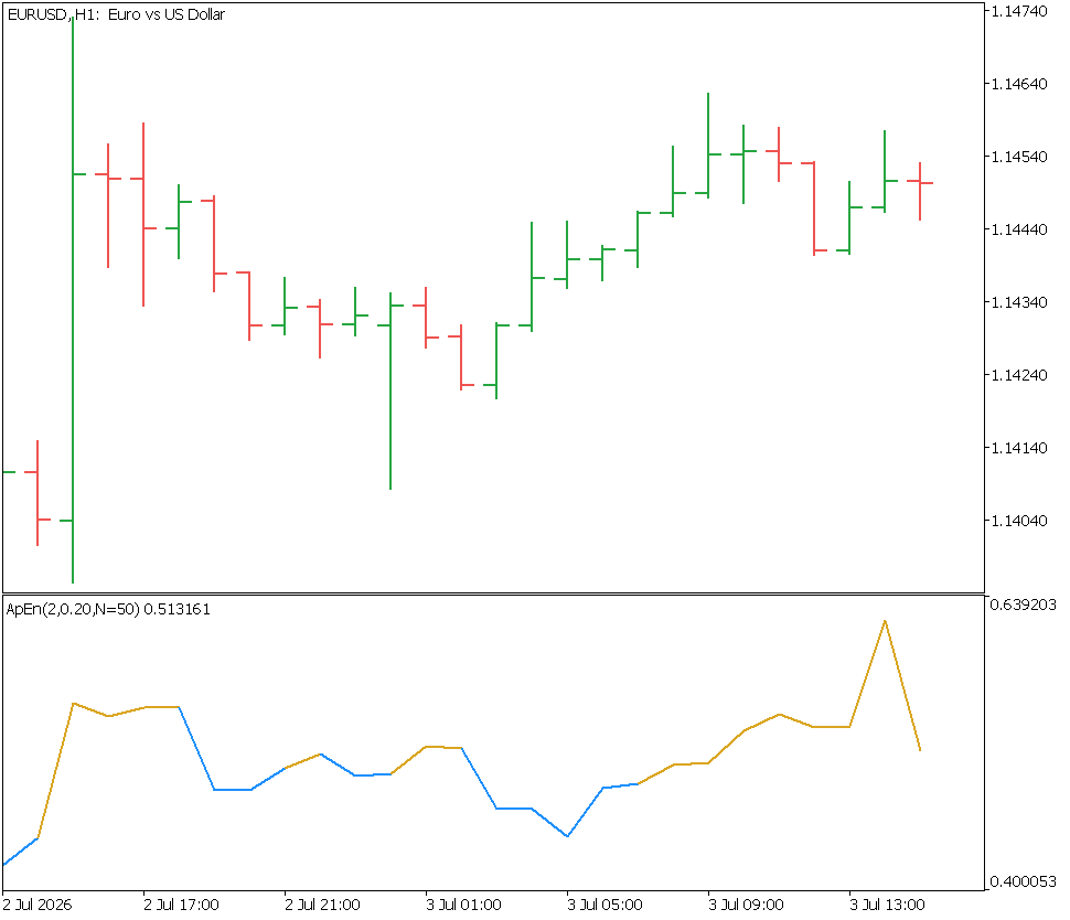
The ApEn(2, 0.20, N=50) oscillator plotted beneath EURUSD H1 price action from 2 Jul to 3 Jul 2026. The line alternates between the structured-zone color (blue, ApEn below the 0.5 low threshold) during the tighter, range-bound stretches on the left and lower-middle of the chart, and the intermediate-zone color (gold, ApEn between 0.5 and 1.2) as the series becomes less structured, most notably during the sustained upward move visible from roughly 3 Jul 05:00 onward. The oscillator never crosses into the red, high-entropy zone in this window, consistent with a 50-bar rolling estimate on an actively trending pair over this particular session.
Section 7: Verification
//+------------------------------------------------------------------+
//|                                                  TestApEn.mq5    |
//+------------------------------------------------------------------+

#property script_show_inputs

#include <ApEn\ApEnCalculator.mqh>

#define ASSERT(cond,msg) \
   if(!(cond)) { PrintFormat("FAIL: %s",msg); } \
   else        { PrintFormat("PASS: %s",msg); }

//+------------------------------------------------------------------+
//| Script program start function                                    |
//+------------------------------------------------------------------+
void OnStart(void)
  {
   int n=100;
   double periodic[];
   double pseudo_random[];
   ArrayResize(periodic,n);
   ArrayResize(pseudo_random,n);

   for(int i=0;i<n;i++)
      periodic[i]=::MathSin(i*0.3);

   ::MathSrand(42);
   for(int i=0;i<n;i++)
      pseudo_random[i]=(double)::MathRand()/32767.0-0.5;

   CApEnCalculator calc_periodic;
   CApEnCalculator calc_random;
   calc_periodic.Init(n,2,0.2);
   calc_random.Init(n,2,0.2);

   for(int i=0;i<n;i++)
      calc_periodic.Push(periodic[i]);
   for(int i=0;i<n;i++)
      calc_random.Push(pseudo_random[i]);

   double apen_periodic=calc_periodic.Compute();
   double apen_random=calc_random.Compute();

   PrintFormat("Periodic series ApEn: %.4f",apen_periodic);
   PrintFormat("Pseudo-random series ApEn: %.4f",apen_random);

   ASSERT(apen_periodic!=EMPTY_VALUE,"Periodic ApEn computed");
   ASSERT(apen_random!=EMPTY_VALUE,"Random ApEn computed");
   ASSERT(apen_periodic<apen_random,"Periodic ApEn lower than random ApEn");
  }
//+------------------------------------------------------------------+
This script constructs two synthetic series of exactly 100 points each, the sample-size guideline derived in Section 3 for m = 2. The periodic series is a discretized sine wave generated with MathSin(), which by construction repeats the same shape over and over and should therefore have low ApEn. The pseudo-random series is generated with MathRand() after seeding with MathSrand() using a fixed seed value of 42, which makes the test's output reproducible from run to run while still producing a series with no deliberate structure. Each series is pushed into its own CApEnCalculator instance, both configured identically with m = 2 and r_factor = 0.2, and Compute() is called on each once the respective window is full.
The ASSERT macro is a simple preprocessor construct that prints either PASS or FAIL followed by a descriptive message, without halting script execution on failure, so all three checks always run and report independently.
The first two assertions simply confirm that both calculators produced a real value rather than EMPTY_VALUE, which would indicate a configuration or sample-size problem. The third and central assertion checks that the periodic series produces a strictly lower ApEn than the pseudo-random series, which is the qualitative behavior the mathematics in Section 2 predicts and which this article's implementation must reproduce to be considered correct. Exact numeric ApEn values are deliberately not asserted, because each series' tolerance r is computed adaptively from its own standard deviation — the sine wave and the uniform pseudo-random series have different SDs, hence different absolute r values, and only the relative ordering (periodic lower than random), not the specific magnitudes, is a property the mathematics guarantees.
Section 8: Using ApEn as a Strategy Gate
The ApEn indicator's output buffer is intended to be consumed by an Expert Advisor as a precondition check before allowing a directional entry, not as a standalone signal generator. A conceptual integration uses iCustom() to attach to the indicator and CopyBuffer() to retrieve the most recently completed value from its main plot buffer (buffer index 0):
double apen_value[];
int handle=iCustom(_Symbol,_Period,"ApEnIndicator",100,2,0.2,0.5,1.2);
if(handle!=INVALID_HANDLE)
  {
   if(CopyBuffer(handle,0,1,1,apen_value)>0)
     {
      if(apen_value[0]<1.2)
        {
         //--- directional entry logic permitted
        }
      else
        {
         //--- directional entry logic gated off
        }
     }
  }
This snippet creates a handle to the custom indicator with the same five parameters discussed throughout the article, then copies a single value starting at shift 1 — the most recently closed bar, not the currently forming bar — into a local array, and checks that value against the high threshold before allowing the EA's own directional logic to proceed.
The shift of 1 rather than 0 is deliberate and important: the indicator's OnCalculate() computes ApEn from the closed-bar log-return series, so the value at shift 0 corresponds to a bar still in progress and is subject to change as the bar continues to form, which would introduce look-ahead-like instability into the gate if used directly. Reading from shift 1 and performing the gate check once per new bar, at bar open, ensures the EA is always gating on a value computed from fully closed price data. This section provides architectural guidance for how such a gate would be wired together; it does not constitute a complete Expert Advisor, and the entry, exit, position-sizing, and risk-management logic that would surround this gate are outside its scope.
Section 9: Limitations
The O(N²) computation underlying every ApEn estimate constrains window size directly: larger windows give more statistically reliable estimates but grow per-bar computational cost quadratically, which in practice keeps the usable range to roughly 50–200 bars for real-time recalculation, as derived in Section 3. ApEn is also known to be biased for short windows — it consistently underestimates the true entropy of the underlying process when N is small, an effect that becomes pronounced below roughly N = 100 for m = 2, meaning the indicator's absolute readings should be interpreted with more caution at the lower end of the recommended window range.
The statistic is sensitive to the choice of r: a different r factor applied to the same return series can produce qualitatively different zone classifications, since r controls how strict the template-matching criterion is, and there is no single "correct" r independent of the application — only conventions, such as 0.2 · SD, that have proven useful in practice.
Critically, a low ApEn reading indicates statistical structure in the return series; it does not by itself indicate a profitable trading opportunity, since detectable structure does not guarantee that the structure is large enough, persistent enough, or directionally exploitable enough to overcome transaction costs — the indicator measures predictability, not edge.
Finally, the indicator as implemented does not perform any significance test: it reports a point estimate of ApEn but does not indicate whether that value is statistically distinguishable from the ApEn of a random series of the same length, which would require a surrogate-data or bootstrap procedure not included in this implementation.
Conclusion
What you now have is a complete, practical ApEn toolkit for MQL5 and a clear workflow for turning predictability estimates into a gate on directional trading:
- A reusable CApEnCalculator includes that computes ApEn over a rolling window with an adaptive r (r = r_factor · SD(window)), exposed via a minimal public API (Init, Push, Compute, IsReady, Reset).
- ApEnIndicator.mq5, a ready-to-use subwindow oscillator that plots ApEn and color-codes three regime zones (structured / intermediate / random) with fully configurable inputs: window size, embedding dimension, r factor, and low/high thresholds.
- TestApEn.mq5, a simple verification script that checks the implementation by asserting a periodic series yields lower ApEn than a pseudo-random series of the same length.
Practical integration checklist (before live use):
- Validate on your instrument/timeframe with TestApEn and with historical replay: different markets have different baseline ApEn ranges.
- In your EA, read the indicator via iCustom and CopyBuffer; copy the most recently closed-bar value (buffer index 0, shift = 1) and use it to gate directional entries (for example: allow entries only if ApEn < high_threshold).
- Tune InpWindowSize, InpRFactor, and thresholds for stability and for your execution costs; prefer N ≥ 100 for m = 2 where feasible.
- Treat a low ApEn as evidence of serial structure (predictability), not as a guarantee of profitability: confirm the directional rule actually monetizes the detected structure after spreads, commissions, and slippage.
- Be aware of limitations: ApEn is O(N²) per update, biased downward for short N, sensitive to r, and the current implementation provides a point estimate without a statistical significance test or surrogate-data bootstrap.
Extensions and next steps:
- Consider SampEn to reduce some bias at the cost of excluding self-matches, Permutation Entropy for faster ordinal-pattern-based estimates, or multiscale entropy for multi-timeframe structure analysis.
- Add a simple bootstrap/surrogate test if you need a statistical significance measure before gating.
By following the verification checklist and tuning the exposed parameters to your market and costs, you can use the provided ApEn implementation as a disciplined, quantitative regime gate that reduces the false-activity of directional EAs when the market offers no measurable short-term predictability.
Programs used in the article:
| # | Name | Type | Description |
|---|---|---|---|
| 1 | ApEnCalculator.mqh | Include File | Maintains a rolling window of return values and computes Approximate Entropy over that window using an adaptive, standard-deviation-scaled tolerance. |
| 2 | ApEnIndicator.mq5 | Custom Indicator | Plots Approximate Entropy as a color-zoned subwindow oscillator computed from closed-bar log-returns, with configurable embedding dimension, tolerance factor, and regime thresholds. |
| 3 | TestApEn.mq5 | Script | Verifies the CApEnCalculator implementation by confirming that a periodic synthetic series produces a lower ApEn value than a pseudo-random synthetic series of the same length. |
| 4 | ApEn.zip | Zip Archive | Zip archive containing all the attached files and their paths relative to the terminal's root folder. |
Warning: All rights to these materials are reserved by MetaQuotes Ltd. Copying or reprinting of these materials in whole or in part is prohibited.
This article was written by a user of the site and reflects their personal views. MetaQuotes Ltd is not responsible for the accuracy of the information presented, nor for any consequences resulting from the use of the solutions, strategies or recommendations described.

 Foundation Models for Trading (Part I): Porting Kronos to Native MQL5
 Building a Synthetic Custom Symbol in MQL5 Using Multi-Symbol Price Averaging
 From Basic to Intermediate: Random Access to Files (I)
 Beyond the Clock (Part 4): Efficacy of Bars on Trending and Mean-Reversion Strategies

- Free trading apps
- Over 8,000 signals for copying
- Economic news for exploring financial markets
You agree to website policy and terms of use