Exponentially Weighted Covariance Matrix in MQL5: Building an Adaptive Correlation Monitor for Multi-Symbol EAs

Introduction

A multi-symbol EA managing correlated positions typically computes its correlation matrix over a fixed historical window and treats every observation inside that window as equally important. This approach has a concrete failure mode. When a correlation regime shifts — for instance, when two currencies that normally move together begin diverging after a central bank announcement — the fixed-window matrix can only incorporate new information as fast as old observations roll out. An EA using a 60-bar window needs all 60 bars to pass before pre-shift readings are fully replaced. During those 60 bars, position sizing and hedging decisions are based on a blended estimate that accurately represents neither the old regime nor the new one.

The operational cost is direct. A pair hedge built on a correlation of 0.85 that has since dropped to 0.30 is no longer a hedge. It is two positions the EA believes are offsetting but are not. Portfolio risk budgeting suffers the same problem: a lagging covariance matrix understates risk at exactly the moment risk is highest.

The solution is an estimator that updates on every bar, overweights recent data, and requires no history buffer. This article builds that estimator and packages it into three components:

• CEWCovariance: exponentially weighted covariance matrix, O(N²) per bar, constant memory
• CHeatmapRenderer: live CCanvas correlation heatmap
• CorrelationMonitorDemo: demo EA for a five-symbol portfolio

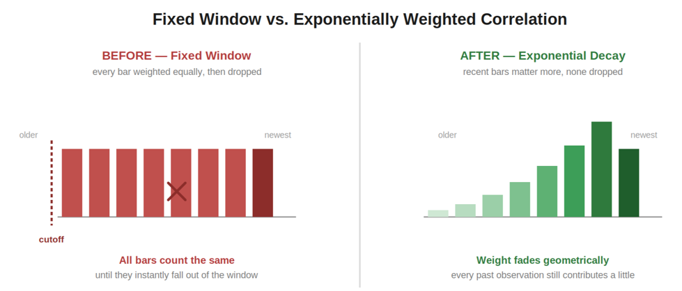
A fixed window weighs every observation equally, then drops it instantly the moment it ages out — a correlation shock takes a full window to fully clear. Exponential decay never drops an observation outright; its influence fades smoothly with age, so recent data always dominates without discarding history completely.

Section 1: The Cost of Static Correlation Windows

A moving window of length W assigns weight 1/W to each of its W observations and zero weight to anything older. If a correlation shock happens at bar t, the estimate does not reflect it fully until bar t+W, when the last pre-shock observation exits. For W = 60 on an H1 chart, that is two and a half days of blended, partially stale estimates driving position sizing decisions.

An exponentially weighted estimator replaces the hard cutoff with a geometric decay. An observation that is k periods old contributes weight λ^k, where λ is a single decay factor between 0 and 1. A shock at bar t immediately influences the very next estimate, weighted by (1 − λ), with that influence fading geometrically as more bars arrive. No observation is ever fully discarded, but older ones carry progressively less weight.

The table below shows effective weights for λ = 0.94:

Periods ago (k)	Weight (1−λ)·λ^k
0	0.0600
1	0.0564
2	0.0530
3	0.0498
4	0.0468
5	0.0440
6	0.0414
7	0.0389
8	0.0365
9	0.0343

The current bar carries more than double the weight of a bar nine periods back. No single observation dominates, but recent data consistently matters more.

Section 2: The Mathematics of Exponential Weighting

The decay factor λ connects to a more intuitive quantity through the effective window formula:

effective_n = 1 / (1 − λ)

This gives the length of a simple moving average with roughly equivalent memory characteristics. For λ = 0.94, effective_n ≈ 16.7, which is the RiskMetrics convention for daily return data. For monthly data, RiskMetrics uses λ = 0.97, giving effective_n ≈ 33.3, since monthly observations are individually noisier and benefit from more smoothing. Increasing λ toward 1.0 extends the effective window and produces slower-adapting, smoother estimates. Decreasing λ toward 0.0 shortens it and produces faster but noisier ones.

The update formula is a single recursive step applied to every matrix entry on each new bar:

Cov(i,j)_t = λ · Cov(i,j)_{t-1} + (1 − λ) · r_i,t · r_j,t

where r_i,t is the return of asset i at time t. The previous estimate is scaled down by λ and a new term is added: the product of the two current returns, weighted by (1 − λ). Only the previous matrix value and the current return vector are needed on each step. There is no stored history and no re-scan, so memory usage stays constant regardless of how long the EA runs.

There is a cold-start problem to account for. At t = 0 the matrix is zero-initialized, and the early updates are dominated by that starting value rather than by real market data. This cold-start bias persists longer than a naive reading of effective_n suggests. With λ = 0.94 and only 5 or 6 observations, individual correlations can swing by several tenths bar-to-bar from estimator noise alone, not from any real market move. The implementation tracks an observation counter and holds a validity flag that only becomes true after a configurable minimum observation count is reached.

Correlation is derived from the covariance matrix by normalizing each off-diagonal entry:

Corr(i,j) = Cov(i,j) / sqrt(Cov(i,i) · Cov(j,j))

This produces a value in [−1, 1] under normal conditions. When either diagonal entry is near zero — meaning the corresponding asset has had near-flat prices and near-zero return variance — the denominator approaches zero and the formula becomes numerically unstable. The implementation checks both diagonal terms against a small epsilon before dividing. Choosing the right epsilon requires care, and Section 4 covers the calibration in detail.

Section 3: MQL5 2D Array Constraints

MQL5 only allows resizing the first dimension of a dynamic 2D array at runtime. The second dimension must be a compile-time constant. This makes a native 2D array declaration unsuitable for a covariance matrix whose size N is determined at runtime by how many symbols are configured.

The workaround used throughout this implementation is to store the matrix as a flat 1D array of length N×N and compute each element's position manually:

index = i * m_n + j

Row i, column j of a logical N×N matrix maps to position i × N + j in the array. Row 0 occupies positions 0 through N−1, row 1 occupies N through 2N−1, and so on. Every method that reads or writes a matrix entry uses a single private helper to compute this index. Developers coming from C++ or Python may not anticipate this constraint since both languages support genuinely dynamic 2D containers.

Section 4: Implementation — EWCovariance.mqh

CEWCovariance owns the running covariance matrix, applies the recursive update on each new observation, and exposes read access to covariance and correlation values. It has no knowledge of rendering or chart objects and can be used in any context, including headless backtests.

//+------------------------------------------------------------------+
//|                                                EWCovariance.mqh  |
//+------------------------------------------------------------------+
#ifndef EWCOVARIANCE_MQH
#define EWCOVARIANCE_MQH

//+------------------------------------------------------------------+
//| Class CEWCovariance                                              |
//| Maintains a running exponentially weighted N x N covariance      |
//| matrix using a flat 1D array with manual index computation       |
//+------------------------------------------------------------------+
class CEWCovariance
  {
private:
   int               m_n;
   double            m_lambda;
   double            m_cov_matrix[];
   int               m_obs_count;
   int               m_min_obs;
   //--- private helper
   int               Index(int i, int j);
public:
                     CEWCovariance(void);
                    ~CEWCovariance(void);
   bool              Init(int n_symbols, double lambda, int min_obs);
   void              Update(const double &returns[]);
   double            GetCovariance(int i, int j);
   double            GetCorrelation(int i, int j);
   bool              IsValid(void);
   void              Reset(void);
   int               GetObsCount(void);
  };

The class holds five members: m_n (symbol count, set at Init time), m_lambda (the decay factor), m_cov_matrix (the flat N×N array), m_obs_count (updated on every successful Update call), and m_min_obs (the warm-up threshold). The private Index helper centralizes the flat-array mapping so the formula appears in exactly one place.

Constructor and Destructor

//+------------------------------------------------------------------+
//| Constructor                                                      |
//+------------------------------------------------------------------+
CEWCovariance::CEWCovariance(void)
  {
   m_n         = 0;
   m_lambda    = 0.0;
   m_obs_count = 0;
   m_min_obs   = 0;
  }
//+------------------------------------------------------------------+
//| Destructor                                                       |
//+------------------------------------------------------------------+
CEWCovariance::~CEWCovariance(void)
  {
  }

m_lambda defaults to 0.0 rather than a conventional value like 0.94. An unconfigured estimator should be visibly inert, not silently computing under an unintended decay assumption. 

The destructor body is empty. m_cov_matrix is a standard MQL5 dynamic array, not a raw pointer or a handle to an external resource, so its memory is reclaimed automatically when the owning object is destroyed; no explicit cleanup call is required. The destructor is still declared and defined explicitly, consistent with the article's style guardrails.

Index()

//+------------------------------------------------------------------+
//| Maps (i,j) onto the flat 1D matrix index                         |
//+------------------------------------------------------------------+
int CEWCovariance::Index(int i, int j)
  {
   return(i * m_n + j);
  }

This single-line helper implements the flat-array mapping from Section 3. Any future change to the memory layout only requires editing this method.

Init()

//+------------------------------------------------------------------+
//| Allocates the matrix and sets estimator parameters               |
//+------------------------------------------------------------------+
bool CEWCovariance::Init(int n_symbols, double lambda, int min_obs)
  {
   if(n_symbols <= 0 || lambda <= 0.0 || lambda >= 1.0 || min_obs < 1)
     {
      ::Print("CEWCovariance::Init - invalid parameters: n=", n_symbols,
              " lambda=", ::DoubleToString(lambda, 4), " min_obs=", min_obs);
      return(false);
     }

   m_n       = n_symbols;
   m_lambda  = lambda;
   m_min_obs = min_obs;

   if(::ArrayResize(m_cov_matrix, m_n * m_n) != m_n * m_n)
     {
      ::Print("CEWCovariance::Init - ArrayResize failed for ", m_n * m_n, " elements");
      return(false);
     }

   ::ArrayInitialize(m_cov_matrix, 0.0);
   m_obs_count = 0;

   return(true);
  }

Init() validates all three parameters before committing any state. Lambda must lie strictly inside (0, 1): a value of 0 discards all history on every step, and a value of 1 never updates at all. Both boundary values make the recursive formula useless. If validation fails, the method logs the offending values and returns false without modifying any existing state. On success, ArrayResize() allocates the flat matrix — the return value is checked against the requested size because ArrayResize() can fail under memory pressure — and ArrayInitialize() zeros every element so the matrix starts from a known state. 

Note that Init() does not enforce any relationship between min_obs and the effective window implied by lambda. A caller can set min_obs far below effective_n, and the class will report Valid: YES on a matrix that has not yet converged. That is a configuration decision left to the caller.

Update()

//+------------------------------------------------------------------+
//| Applies one step of the recursive covariance update              |
//+------------------------------------------------------------------+
void CEWCovariance::Update(const double &returns[])
  {
   if(m_n <= 0 || ::ArraySize(returns) < m_n)
     {
      ::Print("CEWCovariance::Update - matrix not initialized or returns array too short");
      return;
     }

   for(int i = 0; i < m_n; i++)
     {
      for(int j = 0; j < m_n; j++)
        {
         int idx = Index(i, j);
         m_cov_matrix[idx] = m_lambda * m_cov_matrix[idx] +
                             (1.0 - m_lambda) * returns[i] * returns[j];
        }
     }

   m_obs_count++;
  }

Update() applies one step of the recursive formula from Section 2 across all N² entries. The diagonal entries where i equals j accumulate returns[i]², which is exactly the squared-return term that makes Cov(i,i) track variance. The implementation visits every entry including the lower triangle rather than exploiting symmetry, which costs some redundant computation but keeps the code straightforward to verify. The observation counter only increments after a successful update pass, so early returns due to bad input do not advance the warm-up counter.

GetCovariance()

//+------------------------------------------------------------------+
//| Returns Cov(i,j) with bounds checking                            |
//+------------------------------------------------------------------+
double CEWCovariance::GetCovariance(int i, int j)
  {
   if(i < 0 || i >= m_n || j < 0 || j >= m_n)
     {
      ::Print("CEWCovariance::GetCovariance - index out of bounds: i=", i, " j=", j);
      return(0.0);
     }
   return(m_cov_matrix[Index(i, j)]);
  }

GetCovariance() validates both indices before touching the array. An out-of-range request logs a message and returns 0.0. In MQL5 an array-out-of-bounds access at runtime terminates the program, so this check is a safety requirement rather than a convenience.

GetCorrelation()

//+------------------------------------------------------------------+
//| Derives Corr(i,j) from the covariance matrix                     |
//+------------------------------------------------------------------+
double CEWCovariance::GetCorrelation(int i, int j)
  {
   double cov_ii = GetCovariance(i, i);
   double cov_jj = GetCovariance(j, j);

   double denom_sq = cov_ii * cov_jj;
   if(denom_sq < 1.0e-24)
     {
      ::Print("CEWCovariance::GetCorrelation - near-zero variance guard triggered for i=",
              i, " j=", j);
      return(0.0);
     }

   double corr = GetCovariance(i, j) / ::MathSqrt(denom_sq);

//--- clamp for numerical safety against rounding past the theoretical bound
   if(corr > 1.0)
      corr = 1.0;
   else
      if(corr < -1.0)
         corr = -1.0;

   return(corr);
  }

GetCorrelation() implements the normalization formula from Section 2 and checks the denominator product against an epsilon of 1.0e-24 before taking the square root. This epsilon is calibrated for real FX minute-bar log returns, and the calibration matters. A typical M1 log return on a major FX pair is around 10⁻⁵ (a few pips against a price near 1.1). Squared and accumulated through the recursive update, Cov(i,i) for an active symbol settles in the range 10⁻⁹ to 10⁻¹⁰. The product of two such diagonal values therefore lands around 10⁻¹⁸ to 10⁻²⁰ for a healthy symbol pair. An epsilon of 1.0e-12, which looks like a reasonable small number, sits several orders of magnitude above this range and fires on every cell of a live matrix — including the diagonal, which represents a symbol's correlation with itself and should always be exactly 1.0. The value 1.0e-24 sits below the range produced by real trading activity while still catching a genuinely flat or pegged price feed where denom_sq would be at or effectively zero. This epsilon must be re-derived for any instrument class, bar interval, or price scale that differs significantly from minute-bar FX data.

After division, the result is clamped to [−1.0, 1.0]. Floating-point rounding in the covariance recursion can occasionally push a mathematically bounded ratio a few units past the theoretical limits in the last decimal place.

IsValid() and Reset()

/+------------------------------------------------------------------+
//| Reports true once the warm-up threshold has been cleared         |
//+------------------------------------------------------------------+
bool CEWCovariance::IsValid(void)
  {
   return(m_obs_count >= m_min_obs);
  }
//+------------------------------------------------------------------+
//| Zeroes the matrix and resets the observation count               |
//+------------------------------------------------------------------+
void CEWCovariance::Reset(void)
  {
   ::ArrayInitialize(m_cov_matrix, 0.0);
   m_obs_count = 0;
  }

IsValid() returns true only once the observation count has cleared m_min_obs. The matrix produces numeric output from the very first Update call regardless of warm-up status, so IsValid() is what distinguishes a result that has been computed from one that is actually trustworthy. 

Reset() returns the estimator to its post-Init cold-start state — zeroing the matrix and clearing the observation counter — without discarding the configured lambda, n, or min_obs values. This is useful when the trader wants the estimator to re-warm cleanly after a known structural event rather than blending old and new regimes. GetObsCount exposes the raw counter directly so the dashboard can show information like "47 of 30 minimum observations" rather than just a boolean flag.

GetObsCount()

//+------------------------------------------------------------------+
//| Returns the raw observation counter                              |
//+------------------------------------------------------------------+
int CEWCovariance::GetObsCount(void)
  {
   return(m_obs_count);
  }

GetObsCount() is a plain accessor exposing the raw observation count, independent of the IsValid() threshold check. It exists so the heatmap renderer and the demo EA's logging can display "47 of 30 minimum observations" style status information, which is more informative to a trader watching the dashboard than a bare boolean validity flag.

Section 5: The Heatmap Color Model

Correlation values need a visual encoding where both sign and magnitude are immediately readable. The scheme used here is a three-anchor linear interpolation: blue at −1.0, white at 0.0, and red at +1.0.

This is a diverging color scheme. Correlation has a meaningful zero point — a value of 0.0 is qualitatively different from either +1.0 or −1.0, and the visualization needs to reflect that. A simple two-color gradient from blue to red would not create a visually distinct marker for the near-zero region. A white midpoint gives near-zero correlations a clear, high-contrast appearance that a continuous gradient would blur together.

The interpolation is computed in two independent linear segments. For correlation in [−1.0, 0.0], the color blends from blue to white. For correlation in [0.0, +1.0], it blends from white to red. Keeping these as two separate segments with a sign-based switch makes each segment's computation a simple one-parameter blend between two fixed colors.

One MQL5-specific detail requires attention when packing the computed R, G, B byte values into a drawable color. MQL5's color type uses 0x00BBGGRR byte ordering, which matches the Windows COLORREF convention and not the 0xRRGGBB ordering familiar from CSS or most other graphics APIs. Packing bytes as (r << 16) | (g << 8) | b is a common mistake that silently swaps red and blue. The correct packing is (b << 16) | (g << 8) | r. The resulting heatmap looks plausible either way, cells appear in roughly the right positions, so the only reliable check is to verify that the self-correlation diagonal, which must always be exactly +1.0, renders as pure red rather than pure blue.

Section 6: Implementation — HeatmapRenderer.mqh

CHeatmapRenderer handles all drawing: the canvas object, per-cell color computation, axis labels, and status text. It is deliberately separate from CEWCovariance because a canvas creation failure should not prevent the estimator from running, and resetting the estimator should not require touching any drawing code.

//+------------------------------------------------------------------+
//|                                              HeatmapRenderer.mqh |
//+------------------------------------------------------------------+
#ifndef HEATMAPRENDERER_MQH
#define HEATMAPRENDERER_MQH

#include "EWCovariance.mqh"
#include <Canvas\Canvas.mqh>

//+------------------------------------------------------------------+
//| Class CHeatmapRenderer                                           |
//| Draws an N x N correlation heatmap from a CEWCovariance instance |
//+------------------------------------------------------------------+
class CHeatmapRenderer
  {
private:
   CCanvas           m_canvas;
   int               m_n;
   string            m_symbol_names[];
   int               m_cell_size;
   int               m_origin_x;
   int               m_origin_y;
   //--- private helper
   uint              ColorFromCorrelation(double corr);
public:
                     CHeatmapRenderer(void);
                    ~CHeatmapRenderer(void);
   bool              Init(int n, const string &names[], int x, int y, int cell_size);
   void              Render(CEWCovariance &cov, int obs_count, bool is_valid);
   void              Destroy(void);
  };
//+------------------------------------------------------------------+
//| Constructor                                                      |
//+------------------------------------------------------------------+
CHeatmapRenderer::CHeatmapRenderer(void)
  {
   m_n         = 0;
   m_cell_size = 0;
   m_origin_x  = 0;
   m_origin_y  = 0;
  }
//+------------------------------------------------------------------+
//| Destructor                                                       |
//+------------------------------------------------------------------+
CHeatmapRenderer::~CHeatmapRenderer(void)
  {
  }

m_canvas is a member object rather than a pointer, so its own destructor runs automatically when the renderer is destroyed. Explicit removal of the chart bitmap object is handled by Destroy(), which is called from OnDeinit(). Chart object lifetime and C++ object lifetime are not the same thing in MQL5, so this separation is intentional.

Init()

//+------------------------------------------------------------------+
//| Creates the canvas bitmap label and stores layout parameters     |
//+------------------------------------------------------------------+
bool CHeatmapRenderer::Init(int n, const string &names[], int x, int y, int cell_size)
  {
   if(n <= 0 || ::ArraySize(names) < n || cell_size <= 0)
     {
      ::Print("CHeatmapRenderer::Init - invalid parameters");
      return(false);
     }

   m_n         = n;
   m_cell_size = cell_size;
   m_origin_x  = x;
   m_origin_y  = y;

   if(::ArrayResize(m_symbol_names, m_n) != m_n)
     {
      ::Print("CHeatmapRenderer::Init - ArrayResize failed for symbol names");
      return(false);
     }
   for(int i = 0; i < m_n; i++)
      m_symbol_names[i] = names[i];

   int label_margin = 70;
   int canvas_width  = label_margin + m_n * m_cell_size + 20;
   int canvas_height = label_margin + m_n * m_cell_size + 40;

   if(!m_canvas.CreateBitmapLabel("CorrelationHeatmap", x, y, canvas_width, canvas_height,
                                  COLOR_FORMAT_ARGB_NORMALIZE))
     {
      ::Print("CHeatmapRenderer::Init - CreateBitmapLabel failed, error code ", ::GetLastError());
      return(false);
     }

   return(true);
  }

Init() validates inputs, stores layout parameters, and makes a defensive copy of the symbol names array. The canvas size reserves 70 pixels for symbol-name labels along the left and top edges, plus the N×N cell grid, plus a 40-pixel margin below the grid for the status line. A failure from CreateBitmapLabel is logged with GetLastError() and causes Init to return false. The demo EA treats this as fatal and returns INIT_FAILED.

ColorFromCorrelation()

//+------------------------------------------------------------------+
//| Maps a correlation value to an ARGB color                        |
//+------------------------------------------------------------------+
uint CHeatmapRenderer::ColorFromCorrelation(double corr)
  {
   if(corr > 1.0)
      corr = 1.0;
   else
      if(corr < -1.0)
         corr = -1.0;

   uchar r, g, b;

   if(corr < 0.0)
     {
      //--- interpolate blue (corr = -1.0) to white (corr = 0.0)
      double t = corr + 1.0; // 0.0 at corr=-1, 1.0 at corr=0
      r = (uchar)(0   + t * (255 - 0));
      g = (uchar)(0   + t * (255 - 0));
      b = (uchar)(255 + t * (255 - 255));
     }
   else
     {
      //--- interpolate white (corr = 0.0) to red (corr = 1.0)
      double t = corr; // 0.0 at corr=0, 1.0 at corr=1
      r = (uchar)(255 + t * (255 - 255));
      g = (uchar)(255 + t * (0   - 255));
      b = (uchar)(255 + t * (0   - 255));
     }

   return(::ColorToARGB((color)((b << 16) | (g << 8) | r), 255));
  }

For negative correlations, t = corr + 1.0 maps [−1.0, 0.0] linearly onto [0.0, 1.0]. Red and green rise from 0 toward 255 while blue stays fixed at 255, producing a blend from blue to white. For non-negative correlations, t = corr maps [0.0, 1.0] directly. Red stays fixed at 255 while green and blue fall from 255 toward 0, producing a blend from white to red. The bytes are packed as (b << 16) | (g << 8) | r, matching MQL5's 0x00BBGGRR layout described in Section 5. Using the familiar (r << 16) | (g << 8) | b order instead compiles without error and produces a color — just one where red and blue are swapped.

Render()

//+------------------------------------------------------------------+
//| Draws the full N x N heatmap frame                               |
//+------------------------------------------------------------------+
void CHeatmapRenderer::Render(CEWCovariance &cov, int obs_count, bool is_valid)
  {
   m_canvas.Erase(::ColorToARGB(clrWhite, 255));

   int label_margin = 70;
   m_canvas.FontSet("Consolas", 10);

//--- column labels across the top
   for(int j = 0; j < m_n; j++)
     {
      int cx = label_margin + j * m_cell_size + 4;
      m_canvas.TextOut(cx, 4, m_symbol_names[j], ::ColorToARGB(clrBlack, 255));
     }

//--- row labels down the left side
   for(int i = 0; i < m_n; i++)
     {
      int ry = label_margin + i * m_cell_size + (m_cell_size / 2) - 6;
      m_canvas.TextOut(4, ry, m_symbol_names[i], ::ColorToARGB(clrBlack, 255));
     }

   if(!is_valid)
     {
      //--- matrix has not cleared the warm-up threshold yet; draw a neutral
      //--- placeholder grid instead of computing and logging 25 guarded misses
      for(int i = 0; i < m_n; i++)
        {
         for(int j = 0; j < m_n; j++)
           {
            int cell_x = label_margin + j * m_cell_size;
            int cell_y = label_margin + i * m_cell_size;
            m_canvas.FillRectangle(cell_x, cell_y, cell_x + m_cell_size, cell_y + m_cell_size,
                                   ::ColorToARGB(clrGainsboro, 255));
            m_canvas.Rectangle(cell_x, cell_y, cell_x + m_cell_size, cell_y + m_cell_size,
                               ::ColorToARGB(clrGray, 255));
           }
        }
     }
   else
     {
      //--- matrix is warmed up; safe to compute and display every cell
      for(int i = 0; i < m_n; i++)
        {
         for(int j = 0; j < m_n; j++)
           {
            double corr        = cov.GetCorrelation(i, j);
            uint   cell_color  = ColorFromCorrelation(corr);

            int cell_x = label_margin + j * m_cell_size;
            int cell_y = label_margin + i * m_cell_size;

            m_canvas.FillRectangle(cell_x, cell_y, cell_x + m_cell_size, cell_y + m_cell_size, cell_color);
            m_canvas.Rectangle(cell_x, cell_y, cell_x + m_cell_size, cell_y + m_cell_size,
                               ::ColorToARGB(clrGray, 255));

            string cell_text = ::DoubleToString(corr, 2);
            m_canvas.TextOut(cell_x + 6, cell_y + (m_cell_size / 2) - 6, cell_text,
                             ::ColorToARGB(clrBlack, 255));
           }
        }
     }

   int status_y = label_margin + m_n * m_cell_size + 10;
   string status_text = "Observations: " + ::IntegerToString(obs_count) +
                        "   Valid: " + (is_valid ? "YES" : "NO (warming up)");
   m_canvas.TextOut(label_margin, status_y, status_text, ::ColorToARGB(clrBlack, 255));

   m_canvas.Update();
  }

//+------------------------------------------------------------------+
//| Removes the canvas object from the chart                         |
//+------------------------------------------------------------------+
void CHeatmapRenderer::Destroy(void)
  {
   m_canvas.Destroy();
  }

Render() branches on is_valid before touching the correlation matrix. Symbol labels are drawn unconditionally since they do not depend on warm-up state. During the cold-start period, a neutral gray placeholder grid is drawn without calling GetCorrelation() at all. This matters for a practical reason: during cold start, every diagonal variance entry is still near zero. Calling GetCorrelation() would trip the near-zero-variance guard on essentially every cell, on every redraw. With OnTimer() firing every 10 seconds, that generates N² log lines every 10 seconds for as long as warm-up lasts. Skipping the computation entirely during this known state prevents that log flood. Once is_valid becomes true, the second branch computes and fills each cell with its correlation color and numeric label. A status line below the grid reports the raw observation count and validity state on every frame, and m_canvas. Update() flushes the completed bitmap to the chart.

Section 7: Implementation — CorrelationMonitorDemo.mq5

//+------------------------------------------------------------------+
//|                                       CorrelationMonitorDemo.mq5 |
//+------------------------------------------------------------------+

#property strict

#include <EWCovariance/EWCovariance.mqh>
#include <EWCovariance/HeatmapRenderer.mqh>

//--- Input parameters
input string InpSymbol1 = "EURUSD";
input string InpSymbol2 = "GBPUSD";
input string InpSymbol3 = "USDJPY";
input string InpSymbol4 = "XAUUSD";
input string InpSymbol5 = "USDCHF";
input double InpLambda  = 0.94;
input int    InpMinObs  = 30;

//--- Module-scope state
#define N_SYMBOLS 5

string            g_symbols[N_SYMBOLS];
double            g_prev_close[N_SYMBOLS];
datetime          g_last_bar_time[N_SYMBOLS];
CEWCovariance     g_cov;
CHeatmapRenderer  g_renderer;

The five symbols are declared as separate input strings because MQL5's input dialog does not support array-typed inputs. InpLambda and InpMinObs default to 0.94 and 30. The default of 30 sits comfortably above the effective window of approximately 16.7 bars that λ = 0.94 implies, so the Valid flag carries real meaning when it first becomes true.

PrintCorrelationTable()

//+------------------------------------------------------------------+
//| Prints the structured correlation table to the Experts tab       |
//+------------------------------------------------------------------+
void PrintCorrelationTable(void)
  {
   Print("--- Correlation table (obs=", g_cov.GetObsCount(),
         ", valid=", (g_cov.IsValid() ? "true" : "false"), ") ---");
   for(int i = 0; i < N_SYMBOLS; i++)
     {
      for(int j = i + 1; j < N_SYMBOLS; j++)
        {
         double corr = g_cov.GetCorrelation(i, j);
         Print(g_symbols[i], "-", g_symbols[j], ": ", DoubleToString(corr, 4));
        }
     }
  }

PrintCorrelationTable() iterates the upper triangle of the matrix — j starting at i + 1 — to print each of the ten unique pairs among five symbols exactly once. Printing the full N×N grid would duplicate every pair, since Corr(i,j) = Corr(j,i), and would print N meaningless 1.0 self-correlations along the diagonal.

ProcessNewBars()

//+------------------------------------------------------------------+
//| Computes log returns for all five symbols on new bar close       |
//| and feeds them through the covariance update                     |
//+------------------------------------------------------------------+
void ProcessNewBars(void)
  {
   double returns[N_SYMBOLS];
   bool   have_new_bar = false;

   for(int i = 0; i < N_SYMBOLS; i++)
     {
      datetime bar_time = iTime(g_symbols[i], PERIOD_CURRENT, 0);
      if(bar_time != g_last_bar_time[i])
         have_new_bar = true;
     }

   if(!have_new_bar)
      return;

   for(int i = 0; i < N_SYMBOLS; i++)
     {
      double close_now = iClose(g_symbols[i], PERIOD_CURRENT, 1);
      datetime bar_time = iTime(g_symbols[i], PERIOD_CURRENT, 0);

      if(g_prev_close[i] > 0.0 && close_now > 0.0)
         returns[i] = MathLog(close_now / g_prev_close[i]);
      else
         returns[i] = 0.0;

      g_prev_close[i]    = close_now;
      g_last_bar_time[i] = bar_time;
     }

   g_cov.Update(returns);
   g_renderer.Render(g_cov, g_cov.GetObsCount(), g_cov.IsValid());
   PrintCorrelationTable();
  }

ProcessNewBars() is the core per-tick logic, called from OnTick(). It first checks whether any of the five symbols has produced a new bar since the last call, using iTime() on bar index 0 compared directly against the stored g_last_bar_time. Because that baseline is now always a real, non-zero timestamp established in OnInit(), this comparison can be a simple inequality check, with no additional guard needed. This multi-symbol synchronization is approximate, since the five symbols aren't guaranteed to close bars at exactly the same tick. In practice this can mean two or three bar-close events registering within a fraction of a second of each other immediately after attachment, before settling into a steady per-bar cadence — but it's sufficient to gate updates to roughly once per bar interval, rather than on every tick.

If no symbol shows a new bar, the function returns immediately. Otherwise, it computes a log return for each symbol via MathLog(close_now / close_previous), using iClose() on the just-closed bar (index 1, since index 0 is the still-forming current bar). It guards against a zero or unavailable previous close by substituting a 0.0 return rather than dividing by zero, then updates the stored previous-close and bar-time trackers. Finally, it feeds the resulting five-element return vector into g_cov.Update(), redraws the heatmap, and logs the correlation table.

OnInit()

//+------------------------------------------------------------------+
//| Expert initialization function                                   |
//+------------------------------------------------------------------+
int OnInit()
  {
   g_symbols[0] = InpSymbol1;
   g_symbols[1] = InpSymbol2;
   g_symbols[2] = InpSymbol3;
   g_symbols[3] = InpSymbol4;
   g_symbols[4] = InpSymbol5;

   for(int i = 0; i < N_SYMBOLS; i++)
     {
      if(!SymbolSelect(g_symbols[i], true))
         Print("OnInit - warning: could not select symbol ", g_symbols[i]);

      g_last_bar_time[i] = iTime(g_symbols[i], PERIOD_CURRENT, 0);
      g_prev_close[i]    = iClose(g_symbols[i], PERIOD_CURRENT, 1);
     }

   if(!g_cov.Init(N_SYMBOLS, InpLambda, InpMinObs))
     {
      Print("OnInit - CEWCovariance::Init failed");
      return(INIT_FAILED);
     }

   if(!g_renderer.Init(N_SYMBOLS, g_symbols, 10, 10, 60))
     {
      Print("OnInit - CHeatmapRenderer::Init failed");
      return(INIT_FAILED);
     }

   g_renderer.Render(g_cov, g_cov.GetObsCount(), g_cov.IsValid());
   EventSetTimer(10);

   return(INIT_SUCCEEDED);
  }

OnInit() copies the five input symbols into g_symbols, calls SymbolSelect() on each to ensure the terminal has data available, and immediately sets both g_last_bar_time and g_prev_close for every symbol. These baselines must be real values established at attach time, not left at zero. A zero-initialized baseline creates a circular dependency: ProcessNewBars can never detect the first new bar because the code path that would set a real baseline is gated behind having already detected one. Setting real values in OnInit() breaks that dependency. The function then initializes both the estimator and the renderer, returning INIT_FAILED if either fails, draws an initial cold-start frame, and starts a 10-second timer via EventSetTimer().

OnDeinit(), OnTick(), and OnTimer()

//+------------------------------------------------------------------+
//| Expert deinitialization function                                 |
//+------------------------------------------------------------------+
void OnDeinit(const int reason)
  {
   EventKillTimer();
   g_renderer.Destroy();
  }

//+------------------------------------------------------------------+
//| Expert tick function                                             |
//+------------------------------------------------------------------+
void OnTick()
  {
   ProcessNewBars();
  }

//+------------------------------------------------------------------+
//| Timer function - refreshes the heatmap without a new bar         |
//+------------------------------------------------------------------+
void OnTimer()
  {
   g_renderer.Render(g_cov, g_cov.GetObsCount(), g_cov.IsValid());
  }

OnTimer() simply redraws the heatmap every 10 seconds, independent of whether a new bar has occurred. This keeps the "Observations" and "Valid" status fields and any other display elements visibly current, even during a quiet period with no new bar closes. OnDeinit() stops the timer and calls g_renderer.Destroy() to remove the dashboard's chart object cleanly.

The CCanvas heatmap rendered on the active chart for the five-symbol demonstration portfolio (EURUSD, GBPUSD, USDJPY, XAUUSD, USDCHF), showing a 5×5 grid colored per the blue-white-red scheme from Section 5, with each cell annotated by its numeric correlation value, symbol labels on both axes, and a status line reading "Observations: 190   Valid: YES." Every diagonal cell reads exactly 1.00 and renders solid red, confirming both the self-correlation identity and the correct red/blue channel ordering described in Section 5.

Section 8: Verification

The estimator's convergence behavior can be checked without live market data. This is done by feeding it a known synthetic sequence whose theoretical steady-state covariance is computable in closed form, then confirming the reported correlation converges to within a defined tolerance of that closed-form value after enough iterations.

//+------------------------------------------------------------------+
//|                                          EWCovarianceVerify.mq5  |
//+------------------------------------------------------------------+

#property script_show_inputs

#include <EWCovariance/EWCovariance.mqh>

#define ASSERT(cond, msg) \
   if(!(cond)) { Print("FAIL - ", msg); failures++; } \
   else        { Print("PASS - ", msg); }

//+------------------------------------------------------------------+
//| Script program start function                                    |
//+------------------------------------------------------------------+
void OnStart()
  {
   int    failures = 0;
   double lambda   = 0.94;

   CEWCovariance cov;
   if(!cov.Init(2, lambda, 10))
     {
      Print("FAIL - CEWCovariance::Init failed in verification setup");
      return;
     }

//--- synthetic returns with a known target correlation of approximately 0.98 (steady-state EWMA for this periodic input)
//--- asset 0 is the base series, asset 1 = 0.8 * asset0 + small independent noise
   double base_pattern[10] = { 0.010, -0.006, 0.012, -0.004, 0.008,
                               -0.010, 0.006, -0.008, 0.011, -0.005
                             };
   double noise_pattern[10] = { 0.002, -0.001, 0.001, -0.002, 0.001,
                                0.002, -0.001, 0.001, -0.002, 0.001
                              };

   int iterations = 400;
   for(int k = 0; k < iterations; k++)
     {
      int idx = k % 10;
      double r0 = base_pattern[idx];
      double r1 = 0.8 * base_pattern[idx] + noise_pattern[idx];

      double returns[2];
      returns[0] = r0;
      returns[1] = r1;
      cov.Update(returns);
     }

   ASSERT(cov.IsValid(), "estimator reached minimum observation count");

   double corr = cov.GetCorrelation(0, 1);
   double tolerance = 0.01;
   double expected  = 0.9754; // exact steady-state solution of the periodic EWMA recursion

   Print("Converged correlation after ", iterations, " iterations: ", DoubleToString(corr, 4));

   ASSERT(MathAbs(corr - expected) < tolerance,
          "converged correlation within tolerance of expected value");
   ASSERT(corr > 0.0 && corr <= 1.0, "converged correlation within valid bounds");

   double self_corr = cov.GetCorrelation(0, 0);
   ASSERT(MathAbs(self_corr - 1.0) < 0.0001, "self-correlation equals 1.0");

   if(failures == 0)
      Print("VERIFICATION SUMMARY: ALL TESTS PASSED");
   else
      Print("VERIFICATION SUMMARY: ", failures, " TEST(S) FAILED");
  }
//+------------------------------------------------------------------+

Asset 1's returns are constructed as 0.8 times the base series plus small independent noise. The 10-point pattern repeats for 400 iterations, giving the estimator far more than its 10-observation minimum to settle into a steady state.

The expected value of 0.9754 comes from solving the EWMA recursion analytically for a periodic input. When the input repeats with period P, the recursion converges to a periodic limit cycle rather than a single static value. The steady-state covariance at phase p is a weighted sum of the pairwise return products across one full cycle, with weights determined by the geometric decay factor λ. Evaluating this for the specific 10-point pattern at the last processed phase (k = 399, phase 9) gives 0.9754. This is a derived result, not a visual estimate.

The tolerance of 0.01 is tight enough to catch real implementation errors such as a transposed λ and (1 − λ), a wrong loop bound, or a misplaced index. It leaves room for the small oscillation that a periodic limit cycle exhibits between phases and for ordinary floating-point rounding in MQL5's double arithmetic.

The ASSERT macro prints PASS or FAIL per check and increments a counter. The self-correlation check on GetCorrelation(0, 0) is independent of the limit cycle dynamics. Any asset's correlation with itself is a mathematical identity that must hold regardless of decay factor or input series. A failure there points to a bug in the covariance-to-correlation formula itself rather than a calibration issue.

Section 9: Calibrating λ

The effective window formula from Section 2, effective_n = 1 / (1 − λ), gives a direct way to reason about λ in terms a trader is more likely to have intuition for than a raw decay coefficient:

λ	Effective window (bars)
0.90	10.0
0.94	16.7
0.97	33.3
0.99	100.0

The RiskMetrics convention of λ = 0.94 for daily data reflects a judgment that roughly 17 days of effective memory balances responsiveness against noise at daily sampling frequency. It is a widely used starting point, not an optimal value derived from a specific dataset. An EA operating on different timeframes or instruments should treat it as a first approximation and adjust based on observed behavior.

Setting λ too close to 1.0 makes the estimator behave like a near-static long average. At λ = 0.99 the effective window reaches 100 bars, so genuine structural shifts take a long time to register — reintroducing much of the staleness this article was designed to avoid. Setting λ too close to 0.0 produces the opposite problem: the effective window collapses to a few bars and the matrix is dominated by one or two recent observations, making it noisy and sensitive to ordinary single-bar volatility.

min_obs requires the same deliberate attention as λ. Setting it well below effective_n lets the Valid flag become true while the matrix is still heavily influenced by its zero-initialized starting state. At λ = 0.94 with min_obs = 5, individual correlations can swing by several tenths bar-to-bar from estimator noise alone. A min_obs at or above effective_n gives the flag meaningful information when it flips. The article's default of 30 against an effective window of approximately 16.7 is chosen with this in mind.

Section 10: Limitations

The single decay factor λ governs the entire matrix uniformly. A value calibrated for one symbol set or timeframe is not guaranteed to transfer to another. No automated calibration procedure is provided. λ is set once at EA startup via InpLambda and stays fixed unless the EA is restarted or the estimator explicitly reset.

The near-zero-variance epsilon in GetCorrelation is sized for real FX minute-bar log returns. Using this class with a different instrument class, price scale, or bar interval without re-deriving the epsilon risks two silent failure modes. If the epsilon is too large, it fires on legitimate correlations and suppresses them. If it is too small, a genuinely unstable division goes through unchecked. Even when the guard does not trigger, a near-flat asset produces a poorly conditioned correlation row. A tiny but nonzero denominator can amplify numerator noise disproportionately, and the guard does not catch that case.

The implementation displays point-estimate correlations with no confidence measure attached. Two readings of 0.45 and 0.30 appear identically certain on the heatmap, even though the underlying sampling variability of an exponentially weighted estimate depends on both λ and the return distribution. Nothing in the output distinguishes ordinary bar-to-bar noise from a genuine regime shift. This ambiguity is most significant when the estimator has just cleared min_obs and has not yet accumulated substantial weight mass.

The O(N²) matrix update, heatmap render, and correlation table logging all run on MQL5's single processing thread alongside normal tick handling. For five symbols this cost is negligible. The design does not address how it would scale to a much larger symbol universe where per-bar processing time could become a concern.

Conclusion

This implementation presents a complete, constant-memory alternative to lagging fixed-window correlation matrices by combining an online O(N²) covariance engine, a live CCanvas visual grid, and a multi-symbol tracking framework. The design guarantees that structural correlation shifts are captured immediately—weighted by (1−λ) on the very next observation—with adaptive speed governed by a single parameter and a fixed memory footprint independent of session duration.

Conversely, the system operates under specific boundaries: the smoothing factor is fixed manually, the variance guard requires manual recalibration outside of minute FX bars, the minimum-observation threshold must be set relative to the effective window or the validity flag loses meaning, and the system lacks statistical significance testing to isolate true regime shifts from localized sampling noise. To scale this infrastructure, the next logical steps involve implementing dynamic parameter estimation based on observed forecast errors or integrating a Principal Component Analysis module to map dominant risk factors across the portfolio.

Programs used in the article:

#	Name	Type	Description
1	EWCovariance.mqh	Include File	Declares and implements the CEWCovariance class, maintaining a flat-array N×N exponentially weighted covariance matrix with O(N²) per-bar updates and a correlation guard calibrated for real FX return magnitudes.
2	HeatmapRenderer.mqh	Include File	Declares and implements the CHeatmapRenderer class, rendering a CCanvas-based blue-white-red correlation heatmap with correctly channel-ordered colors, axis labels, and a cold-start-aware placeholder state.
3	CorrelationMonitorDemo.mq5	Demo EA	Demonstrates the estimator and renderer on a five-symbol portfolio, establishing a real per-symbol baseline at attach time, computing log returns on each new bar, updating the covariance matrix, redrawing the heatmap, and logging a structured correlation table.
4	EWCovarianceVerify.mq5	Script	Verifies the estimator's convergence behavior against a synthetic two-asset periodic return series, asserting convergence to a closed-form derived correlation within a tight, justified tolerance.
5	EWCovariance.zip	Zip Archive	Zip archive containing all the attached files and their paths relative to the terminal's root folder.