Beyond the Clock (Part 4): Efficacy of Bars on Trending and Mean-Reversion Strategies

Table of Contents

1. Introduction
2. The Volume Problem on Spot FX
3. Why Bar Type Is a Confound, Not a Free Choice
4. The Theory Being Tested
5. Experimental Design
6. Building the Bars on a Common Cadence
7. Primaries and a Directionality Trap
8. Meta-Labeling the Entries
9. Sampling Uniqueness and the Corrected Forest
10. Scoring Under Purged Cross-Validation
11. Statistical Properties on Real EURUSD
12. Results
13. Statistics Versus Efficacy
14. The Grid Is a Multiple-Testing Problem
15. From Python to MQL5
16. Conclusion
17. Attached Files

Introduction

The first three articles in this series built the machinery for alternative bars: Part 1 constructed activity and imbalance bars, Part 2 added runs bars, and Part 3 built an indicator to watch them form inside the terminal. Across all three, one claim was taken on trust. López de Prado argues in Section 2.3 of Advances in Financial Machine Learning that alternative bars (sampled by trading activity or order-flow imbalance rather than by the clock) have better statistical properties than fixed clock-time bars. The unstated corollary, repeated throughout the retail literature, is that strategies and machine-learning models built on those bars must therefore perform better.

That corollary is asserted far more often than it is measured. Better-conditioned returns are a property of the sampling; they do not automatically become a property of a strategy run on top of the sampling. An RSI rule does not know which bar clock produced its inputs. Whether the change of representation helps it is an empirical question that has to be answered with a controlled experiment, not a citation.

This article runs the experiment on 60.5 million EURUSD quote ticks from 2022–2023. Over that period, EURUSD fell from 1.15 through parity and later moved back above 1.10, covering both trending and mean‑reverting regimes. On each bar representation, three classic primaries are run: RSI and Bollinger Bands (mean-reversion) and an ADX/DI rule (trend-following). Every entry is labeled with the triple-barrier method, and a meta-model is trained to learn when to take the primary's bet. Efficacy is summarized by two numbers per cell: the primary's raw hit rate and the meta-model's out-of-sample AUC under purged cross-validation.

The corrected experiment reaches a blunt conclusion. No bar family produces a reliable edge for these rules. Every out-of-sample AUC sits in a narrow band from 0.42 to 0.55, the ordering of families by statistical conditioning does not predict their ordering by efficacy, and a Monte Carlo permutation test on the single best-looking cell returns a p-value of 0.10. The apparent structure in the grid is indistinguishable from what random labels would produce. The statistical property López de Prado documents is real, and this article confirms it on real EURUSD, but it does not carry through to strategy efficacy the way the retail corollary assumes.

The Volume Problem on Spot FX

Before any comparison can be trusted, one problem specific to foreign exchange has to be settled. Six of the ten AFML bar types are defined in terms of traded volume: volume bars, dollar bars, and the volume and dollar variants of the imbalance and runs families. Spot FX is decentralized. There is no consolidated tape and no true market volume, and a retail MetaTrader feed or a Tick Data Suite export reports only quotes. The 2022 and 2023 exports used here carry exactly two columns, bid and ask, with no volume field at all.

The usual workaround is to substitute a unit of tick count for each trade, so that "volume" becomes the number of quote updates. This quietly destroys the distinction the volume and dollar bars were meant to draw. A volume bar closes after a fixed cumulative volume; with one unit per tick, that is a fixed tick count, which is a tick bar. A dollar bar closes after a fixed cumulative price times volume; with one unit per tick, that is a fixed sum of prices, which is a tick bar modulated only by the slowly-moving price level. The table below reports the coefficient of variation of ticks per bar, where zero means a perfectly regular bar and therefore a tick bar.

Bar type (unit volume)	CV of ticks per bar	Meaning
tick	0.000	reference (regular by construction)
volume	0.000	identical to a tick bar
dollar	0.040	a tick bar with a 4% price-level wobble

The imbalance and runs families collapse the same way. A tick-imbalance bar uses only the tick-rule sign sequence, so it stays distinct. Its volume and dollar variants multiply that sign by size or by value, and with a unit per tick they reduce back to the tick variant. The ten AFML bar types therefore collapse to four genuinely distinct families on spot-FX quote data: time, tick, tick-imbalance, and tick-runs.

There is a deeper point here than a missing column. López de Prado motivates dollar bars in Section 2.3.1.4 with two arguments specific to equities: normalizing for large price appreciation, and robustness to changes in shares outstanding from corporate actions. FX spot has neither. There are no shares outstanding, no splits or buybacks, and the price level of a major pair moves within a narrow band. Even with a true volume feed, dollar bars would add little over volume bars for a currency pair. On spot FX the construct is a solution to a problem the market does not have, and the label "dollar bar" describes a price-weighted tick bar.

Why Bar Type Is a Confound, Not a Free Choice

The naive way to compare bar types is to pick a threshold for each, run the strategy, and compare returns. This is broken before it starts, because changing the bar type changes two things at once. A tick bar of one size and a one-hour time bar over the same history produce different numbers of bars, and they also produce bars with different serial-correlation structure. Any difference in downstream performance is then a tangle of sample-size effects and representation effects, and the two cannot be separated after the fact.

The fix is to hold the number of samples constant and vary only the representation. Every family here is calibrated to roughly twelve thousand bars over the two years, so a difference in meta-model AUC between two families can be attributed to representation rather than to one cell training on more data. The realized cadence still fluctuates, and that fluctuation is the phenomenon under study, but its mean is pinned to a shared reference.

The Theory Being Tested

López de Prado's case is statistical, and it pays to be precise about where the book makes that case. Section 2.3.1 covers the standard activity bars (tick, volume, dollar); Section 2.3.2 covers the information-driven bars (imbalance and runs). The explicit evidence for better conditioning sits in the first group. Following Mandelbrot and Taylor (1967) and Ané and Geman (2000), sampling as a function of trading activity yields returns closer to independent and identically distributed Gaussian, with weaker serial correlation than time bars exhibit. For the information-driven bars of Section 2.3.2 the same superiority is asserted and posed as end-of-chapter exercises rather than demonstrated. That gap between what is shown and what is claimed is part of what this article closes.

None of this is controversial as a statement about return distributions. The leap worth scrutinizing is the one to strategy efficacy. A meta-model's job is to separate the primary's profitable signals from its unprofitable ones. Whether information-driven sampling makes that separation easier depends on whether the primary's edge, and the features that predict it, survive the change of clock. A trend rule, whose edge lives in price runs, and a mean-reversion rule, whose edge lives in price overshoots, may respond to the same resampling in opposite directions. That is the hypothesis the grid is built to expose.

Experimental Design

The harness holds everything fixed except the one factor under test. Within each (strategy, labeling) cell, the bar representation is the only thing that changes. The feature set, the volatility target, the barrier widths, the meta-model, and the cross-validation protocol are identical across families. This is what makes the comparison interpretable.

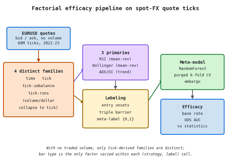
Figure 1. Five-stage illustration of the factorial efficacy pipeline

• Quote stream: 60.5 million bid/ask ticks with no volume field; they feed everything downstream, so every family sees identical raw information.
• Four distinct families: time, tick, tick-imbalance, and tick-runs; the volume and dollar variants collapse onto tick and are excluded.
• Three primaries: RSI and Bollinger (mean-reversion) and ADX/DI (trend-following) generate the side of each bet.
• Labeling: entries are sampled, run through the triple-barrier method, and reduced to a binary meta-label in {0, 1}.
• Meta-model and efficacy: a uniqueness-controlled random forest is scored under purged k-fold CV, and its efficacy is compared against the return-conditioning statistics.

Building the Bars on a Common Cadence

The mid-price drives every bar. Time bars close on the hour; tick bars close on a fixed count calibrated to match that cadence; the tick-imbalance and tick-runs thresholds are calibrated to the same target so the four families carry comparable bar counts.

for bt in BAR_TYPES:  # time, tick, tick_imbalance, tick_runs
    if bt == "time":
        b = make_bars(ticks, bar_type="time", bar_size="H1", price="mid_price")
    elif bt == "tick":
        b = make_bars(ticks, bar_type="tick", bar_size=size, price="mid_price")
    else:  # information bars auto-calibrate to the cadence
        b = make_bars(ticks, bar_type=bt, target_timeframe="H1",
                      ewm_span=EWM_SPAN, price="mid_price")
    bars[bt] = b

One subtlety carries through the whole study. With quote-only data, the tick rule reflects the direction of mid-price updates rather than the trade aggressor side (which is unobservable here). On this data the resulting sign is almost perfectly balanced, at a buy proportion of 0.499, because quote revisions carry very little persistent order-flow imbalance. The tick-imbalance and tick-runs bars are still well-defined, but their informational rationale, which rests on trade-flow persistence, is weakened on quote-only data. That weakening is one of the things the results make visible.

Primaries and a Directionality Trap

Two of the three primaries are mean-reversion rules; the third is trend-following. The trend rule hides a trap worth spelling out, because it is a mistake that propagates silently into the meta-model.

ADX measures trend strength, not direction. A high ADX says a trend is present; it says nothing about whether to buy or sell. A meta-labeling primary, by contrast, must emit a side, because the meta-model's entire job is to decide whether to take that side's bet. Reading an ADX or ADXR crossover as a buy or sell signal, as a naive implementation invites, feeds the meta-model a direction the indicator never actually defined. The correct construction takes the side from the +DI/−DI relationship and uses ADX only as a strength gate. The directional component comes from the Directional Movement System; ADX filters it.

def primary_side(strategy, bars_df):
    sig = strategy.generate_signals(bars_df).astype("float64")
    if type(strategy).__name__ == "DirectionalMovementStrategy":
        # hold the trend, don't re-open only on the crossover bar
        sig = sig.replace(0, np.nan).ffill().fillna(0)
    return sig.astype("int8")

The forward-fill matters too. A bare crossover fires on a single bar; a position is something you hold while the trend persists. Forward-filling the side turns the crossover into a held state, which is both more realistic and the reason the trend cells carry three times as many events as the mean-reversion cells.

Meta-Labeling the Entries

For meta-labeling, events are the rule's own entries. Each onset is included, along with periodic re-assessments while the signal persists. This is applied uniformly across strategies so that cells differ only by representation. Each event is run through the triple-barrier method. get_events walks price forward to the first touch of the volatility-scaled profit-take, stop-loss, or vertical barrier, and get_bins, given the primary's side, returns a label in {0, 1}, one if the bet would have won and zero otherwise. That binary outcome is the meta-model's target.

vbar = add_vertical_barrier(t_events, close, num_bars=VBAR)
events = get_events(close=close, t_events=t_events, pt_sl=PT_SL, target=vol,
                    min_ret=0.0, vertical_barrier_times=vbar,
                    side_prediction=side.reindex(t_events))
binned = get_bins(events, close)  # bin in {0,1} = meta-label

The feature set is intentionally small and shared across every cell: RSI, the Bollinger z-score, ADX, the +DI/−DI spread, the last bar return, an EWM volatility estimate, and tick count per bar. Holding the features fixed is what isolates the bar representation as the active variable. If each strategy carried bespoke features, a difference between cells could not be attributed to the bar clock.

Sampling Uniqueness and the Corrected Forest

Triple-barrier labels overlap. An event opened at bar t may not resolve until bar t + 20, and every event that opens in between shares part of its outcome window. The observations are therefore not independent, and a random forest that draws a full bootstrap of size N from them draws near-duplicate rows. Its trees become correlated, and the covariance term in the AFML §6.2 error decomposition stops shrinking no matter how many trees are added. Bagging only reduces variance when its base learners are decorrelated.

The fix comes from AFML §4.5 and §6.3. Average uniqueness measures how non-overlapping a label set is: for each bar, uniqueness is one over the number of concurrent events, and a sample's uniqueness is the mean of that quantity over its lifespan. Setting the forest's max_samples to average uniqueness makes each tree draw only the effective (non-redundant) number of rows instead of the full N. The class weights are rebalanced on each bootstrap draw with balanced_subsample, which is valid on the forest estimator but not on a bare decision tree.

from afml.sampling.concurrent import get_av_uniqueness_from_triple_barrier

def cell_uniqueness(t1, close):
    # mean of the per-event average uniqueness (AFML Snippet 4.4)
    events = pd.DataFrame({"t1": t1})
    u = get_av_uniqueness_from_triple_barrier(events, close, num_threads=1, verbose=False)
    return float(u["tW"].mean())

def meta_forest(max_samples):
    # AFML 4.5 / 6.3: draw only avgU of the rows per tree; rebalance per draw
    return RandomForestClassifier(
        n_estimators=300, max_samples=max_samples, class_weight="balanced_subsample",
        criterion="entropy", max_features="sqrt", n_jobs=-1)

The uniqueness of a cell is a property of its events, not of the bar type alone, and the values below make one design decision visible. The stateful ADX/DI rule holds a position across the whole trend, so its events overlap heavily and its uniqueness is low, near 0.38. The mean-reversion rules fire in short, separated episodes, so their events overlap little and their uniqueness is high, near 0.63. The forest draws proportionally fewer rows per tree in the ADX/DI cells, which is exactly the correction the overlap calls for.

Bar family	RSI	Bollinger	ADX/DI
time	0.634	0.649	0.366
tick	0.624	0.649	0.380
tick-imbalance	0.609	0.647	0.379
tick-runs	0.651	0.664	0.383

Scoring Under Purged Cross-Validation

The same overlap that motivates the uniqueness correction also breaks naive cross-validation. A label whose window straddles the boundary between a training fold and a test fold leaks its outcome across the split. PurgedKFold removes training observations whose label window overlaps the test set and applies an embargo after each fold. AUC is scored on predict_proba, the quantity that drives bet sizing downstream.

def purged_auc(X, y, t1, max_samples, n_splits=5, embargo=0.01):
    cv = PurgedKFold(n_splits=n_splits, t1=t1, pct_embargo=embargo)
    aucs = []
    for train, test in cv.split(X):
        clf = meta_forest(max_samples).fit(X.iloc[train], y.iloc[train])
        p = clf.predict_proba(X.iloc[test])[:, 1]
        aucs.append(roc_auc_score(y.iloc[test], p))
    return np.mean(aucs)

Statistical Properties on Real EURUSD

The first thing to check is whether López de Prado's statistical claim even holds on this data. It does, and cleanly, for the standard activity bars.

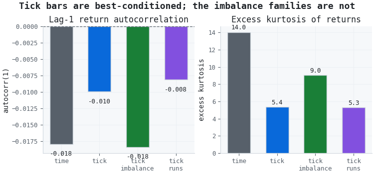
Figure 2. Two-panel illustration of return conditioning by bar family

• Panel (a): lag-1 return autocorrelation. All four families sit close to zero; time bars carry the largest residual at −0.018.
• Panel (b): excess kurtosis. Tick and tick-runs bars cut the fat tails of time bars by more than half, from 14.0 down to about 5.3.

The activity bars win on conditioning, exactly as Section 2.3.1 predicts. The information-driven family does not extend the gain. Tick-imbalance bars carry an excess kurtosis of 9.0, worse than plain tick and tick-runs bars, because the sign they accumulate is quote-driven and almost balanced rather than trade-driven and persistent. The best-conditioned families on this data are the two simplest tick-derived ones.

Results

The efficacy grid pairs each of the four families with each of the three primaries.

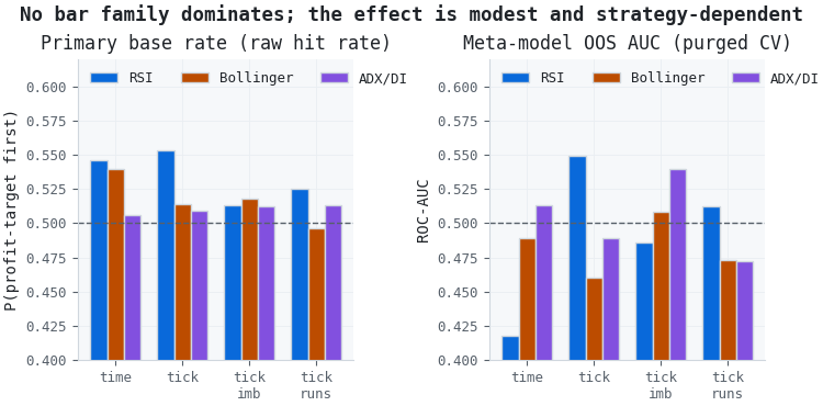
Figure 3. Two-panel illustration of bar-family efficacy by strategy

• Panel (a): the primary base rate, or raw hit rate. Every cell sits near the 0.50 line, between 0.50 and 0.55, with no family systematically ahead.
• Panel (b): the meta-model's out-of-sample AUC under purged CV. Every cell falls between 0.42 and 0.55, straddling the 0.50 line of no skill, with no family clearly above it.

The effect of bar representation is small and it is not systematic. The family means cluster tightly: 0.47 for time, 0.50 for tick, 0.51 for tick-imbalance, and 0.49 for tick-runs. The single highest cell is tick with RSI at 0.550, and the single lowest is time with RSI at 0.418, so the within-strategy spread across families is of the same order as the noise. The raw base rate tracks none of this. It sits near a coin flip everywhere, which is expected for classic rules whose edge, if any, is in which signals to take rather than in the average signal.

Statistics Versus Efficacy

Placing the two measurements on the same axes makes the central finding explicit. The horizontal axis is return conditioning, where lower excess kurtosis is what López de Prado's argument calls better. The vertical axis is efficacy, the meta-model AUC averaged over the three strategies.

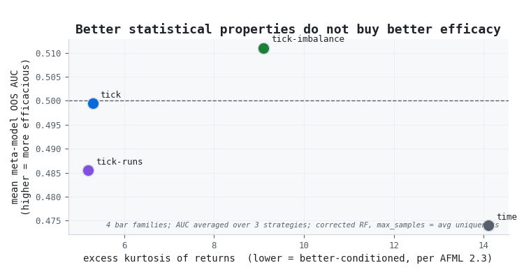
Figure 4. Single-panel illustration of conditioning against efficacy for the four families

If the retail corollary held, the points would fall along a downward line, with better conditioning on the left buying higher efficacy at the top. They do not. The two best-conditioned families, tick and tick-runs near a kurtosis of five, land at efficacies of 0.50 and 0.49. The worst-conditioned family, time near a kurtosis of fourteen, lands lowest at 0.47, and the middling tick-imbalance family lands highest at 0.51. The four points scatter within a range of 0.04 on the efficacy axis with no relationship to the conditioning axis. Return conditioning explains none of the efficacy spread, and the spread itself is small enough to demand a significance test before it is read as anything at all.

The Grid Is a Multiple-Testing Problem

Twelve cells were evaluated, four families times three primaries, and the notebook builds all ten AFML bar types, then sets aside the six volume/dollar variants as duplicates on quote-only FX data. The best cell will look good by construction. That is data-mining bias, the central concern of Aronson's Evidence-Based Technical Analysis and the reason White devised the Reality Check. The right response is to test the best cell against the distribution of what the same pipeline produces on meaningless labels.

We run a Monte Carlo permutation test on the winning cell, tick with RSI. The label column is shuffled, the full purged-CV pipeline is re-fit, and the resulting AUC is recorded; repeating this 200 times builds the null distribution of AUC under no real association.

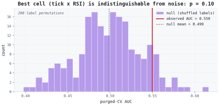
Figure 5. Single-panel illustration of the permutation null for the best cell

The observed AUC (0.550) lies within the bulk of the null distribution (mean 0.499, SD 0.039). The permutation p-value is 0.10. The best cell in the entire grid is not significant at the 0.05 level even before any correction for the twelve tests, and a Šidák adjustment would push the required threshold below 0.005. Nothing in this grid survives that bar. The honest reading is that bar representation, for these classic rules on spot-FX quote data, produces no efficacy edge that can be distinguished from noise.

From Python to MQL5

The study runs in Python because the factorial sweep is a research task rather than a production workload. Deployment uses the MQL5 machinery built earlier in this series. BarBuilderEA constructs the winning bar type live from the tick stream (Parts 1 and 2), and AlternativeBarsViewer (Part 3) lets the calibration be watched in the terminal before any model sees the data, so the same degenerate-bar check that protects the offline feature pipeline protects the live one. The meta-model exports to ONNX, and the primary's side and the secondary's probability drive position sizing through bet_size_probability.

In production the lean harness above is replaced by ModelDevelopmentPipeline, which handles preprocessing, hyperparameter optimization, calibration, and artifact management. The primary trains with is_primary=True and hands its events to the secondary through prepare_meta_labeling_inputs(); the secondary trains with is_primary=False. Switching the deployed representation is a one-line change to the bar_type field of the pipeline's data configuration.

Conclusion

Information-driven bars do have the better statistical properties López de Prado documents, and this article confirmed it on real EURUSD: tick bars cut the excess kurtosis of time bars by more than half. What the article measures is the next link in the chain, whether those properties translate into efficacy for the classic indicators traders actually run. On two years of EURUSD they do not. Every family sits near the no-skill line, conditioning does not predict efficacy, and the best-looking cell fails a permutation test.

Two lessons carry beyond EURUSD. The first is that on spot FX, where no traded volume exists, six of the ten AFML bar types collapse onto tick bars, and dollar bars in particular solve an equities problem the currency market does not have. The second is methodological: equalize the sample sizes before comparing, control the bootstrap for label overlap, purge the cross-validation, and account for multiple testing with a permutation test before believing any winner. The statistical case for alternative bars is sound. The efficacy case, for classic rules on spot FX, is not made by the data. The next article turns from the bar representation to the ensemble itself and asks whether sequential bootstrapping, rather than the uniqueness-controlled forest used here, changes that verdict.

Attached Files

The afml/ folder is a minimal excerpt of the Blueprint Quant afml package: only the subpackages this notebook imports, with empty package markers in place of the full package's loader. It requires numba, scipy, statsmodels, and TA-Lib alongside numpy, pandas, and scikit-learn.

	File	Location	Description
1.	BeyondTheClock_Part4_Efficacy.ipynb	Notebooks\	Reproducible notebook. Builds the four bar families from the 2022-2023 quote ticks, computes average uniqueness, runs the efficacy grid with the uniqueness-controlled forest, and reproduces the permutation test and every figure in the text.
2.	afml/data_structures/	afml\	make_bars and the standard, information, and calibration bar builders that resample ticks into the four families.
3.	afml/strategies/	afml\	RSI, Bollinger, ADX, and Directional-Movement primary strategies that generate each cell's side.
4.	afml/labeling/	afml\	Triple-barrier labeling (add_vertical_barrier, get_events, get_bins) and trend scanning.
5.	afml/sampling/	afml\	get_av_uniqueness_from_triple_barrier for the max_samples value, plus the sequential bootstrap used in Part 5.
6.	afml/cross_validation/	afml\	PurgedKFold and the scoring helpers used to score the meta-model without label leakage.
7.	afml/ensemble/, filters/, util/, sample_weights/	afml\	SequentiallyBootstrappedBaggingClassifier, the CUSUM filter, the volatility target, and sample-weight helpers.