

Implementing Walk-Forward Efficiency Ratio Scoring in MQL5 to Detect Over-Optimized Strategies
 2 222
2 222
 0
0

Introduction
Every algorithmic developer eventually encounters the curve-fitting paradox: an expert advisor that achieves an exceptional equity curve in the MetaTrader 5 Strategy Tester, only to collapse on a live server. This occurs when optimization captures localized historical noise instead of persistent market inefficiencies. The more flexible your parameters, the easier it is for the optimizer to build an illusion of profitability.
Walk-Forward Analysis (WFA) conceptually addresses this by splitting data into in-sample optimization windows and out-of-sample forward tests. However, manual validation does not scale. Visual inspection of fragmented equity curves cannot provide an objective framework for risk management. We need a systematic evaluation pipeline that converts out-of-sample performance degradation into an absolute, reproducible metric.
This implementation changes that by introducing a programmatic scoring architecture built entirely in native MQL5. At the center of this engine is the Walk-Forward Efficiency (WFE) score, which maps the OOS-to-IS Sharpe ratio distribution.
The pipeline components include:
- Data Logging: A companion EA that captures precise per-bar equity changes during backtesting.
- Ingestion Layer: A dedicated CSV reader module designed to parse trade-log metrics efficiently.
- Visualization Engine: A dynamic, color-coded histogram built with the native CCanvas library for instant diagnostic feedback.
To prove the framework provides objective validation rather than confirmation bias, we run the pipeline against two distinct five-year EURUSD Daily data setups — contrasting an over-optimized Moving Average strategy with a theoretically rigid counterpart.
Section 1: The Epistemology of Overfitting
MetaTrader 5's Strategy Tester ranks parameter combinations by a fitness criterion — net profit, Sharpe ratio, or a custom metric. The mathematics of this ranking guarantees a specific failure mode. As the number of free parameters k grows relative to the number of independent observations n in the optimization window, the optimizer increasingly fits the random residuals of the historical price path rather than any persistent structural signal.
The degrees of freedom consumed by the fit are:
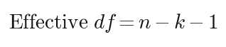
When k approaches n, the in-sample equity curve becomes smooth not because the strategy discovered an edge, but because parameter flexibility allowed the optimizer to reconstruct the historical path. The signature of this regime is a sharp performance discontinuity at the in-sample/out-of-sample boundary: in-sample Sharpe ratios of 2.0–3.0 collapsing to near zero or negative on forward data the optimizer never observed.
Walk-Forward Analysis (WFA) measures this directly. The dataset (length T) is split into W sequential segments. Each segment contains an in-sample window ISw (length L_IS) followed by an out-of-sample window OOSw (length L_OOS). For a rolling configuration, segment w spans:


The core diagnostic is the Walk-Forward Efficiency, the ratio of out-of-sample to in-sample Sharpe for each segment:
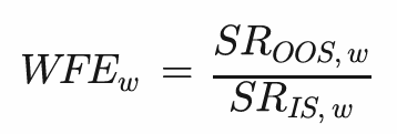
A value near 1.0 means the parameter set transferred its performance to forward data intact. A value near 0 means the in-sample performance was largely artificial. A negative value means the parameters reversed direction out-of-sample. The robustness threshold used throughout this implementation is:

A window retaining at least half its in-sample efficiency is treated as the minimum bar for robustness.
Section 2: The Sharpe Ratio and Its Boundary Conditions
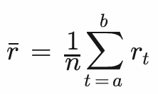
For a return slice r[a..b] of length n = b - a + 1, the annualized Sharpe ratio is computed in three steps:
Step 1 — arithmetic mean of returns:
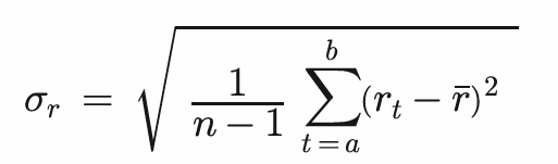
Step 2 — sample standard deviation (Bessel-corrected):
Step 3 — annualized Sharpe:
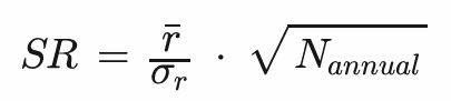
The annualization factor N_annual depends on bar frequency: 252 for daily, 1512 for H4, 6048 for H1, 24192 for M15. Dividing by n-1 rather than n in the standard deviation avoids downward bias in small windows.
The WFE ratio has two boundary conditions that, if ignored, produce misleading scores.
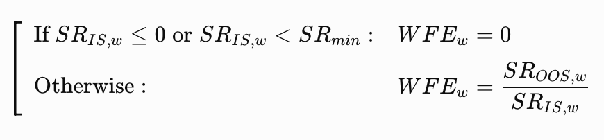
Non-positive in-sample Sharpe: If SR_IS ≤ 0, the window must be flagged as failure unconditionally:

This single rule handles two distinct traps. First, an optimizer should never select a negative-IS parameter set, so encountering one signals data corruption or a catastrophic optimizer configuration. Second, and more subtly, when both SR_IS and SR_OOS are negative, naive division yields a positive WFE — a false pass for a strategy that lost money in both windows. Gating on SR_IS ≤ 0 eliminates both.
Near-zero in-sample Sharpe: When SR_IS is positive but tiny, the division denominator approaches zero and WFE diverges to arbitrarily large values. A window with SR_IS = 0.003 is statistical noise, not a high-quality calibration. A minimum IS Sharpe magnitude SR_min (set to 0.25) is therefore required, below which the window is treated as failure:
Section 3: Building the Computation Engine
The engine lives in a single header, WFE_Engine.mqh. It is built in the order a reader needs to understand it: first the data types it operates on, then each computation that consumes those types, and finally the function that orchestrates them.
The Data Types
Before any computation, two types are needed: an enumeration of annualization factors, and a record holding everything computed about a single walk-forward window.
//+------------------------------------------------------------------+
//|                                                   WFE_Engine.mqh |
//|             Walk-Forward Efficiency Computation Library          |
//+------------------------------------------------------------------+
#ifndef WFE_ENGINE_MQH
#define WFE_ENGINE_MQH

//--- Annualization multipliers based on approximate standard trading periods per year
enum ENUM_TRADE_FREQUENCY
  {
   FREQ_DAILY = 252,          // ~252 trading days per year
   FREQ_H4    = 1512,         // 6 sessions per day * 252
   FREQ_H1    = 6048,         // 24 hours * 252
   FREQ_M15   = 24192         // 96 periods per day * 252
  };

//--- Struct to track performance metrics for a single rolling window step
struct WFERecord
  {
   int                is_start;      // In-Sample start bar index
   int                is_end;        // In-Sample end bar index
   int                oos_start;     // Out-of-Sample start bar index
   int                oos_end;       // Out-of-Sample end bar index
   double             sr_is;         // Annualized In-Sample Sharpe Ratio
   double             sr_oos;        // Annualized Out-of-Sample Sharpe Ratio
   double             wfe;           // Walk-Forward Efficiency score
   bool               is_pass;       // Window met or exceeded pass threshold
   bool               is_valid;      // Metrics calculation successfully processed
  };
The enumeration assigns each timeframe its annual period count directly as the enum value, so the integer behind FREQ_DAILY is literally 252. This lets the calling code pass the enum and have it interpreted as a number without a lookup table.
WFERecord is the output unit. It stores window boundaries (is_start...oos_end), Sharpe ratios (sr_is, sr_oos), the WFE score (wfe), the pass flag (is_pass), and validity (is_valid). Separating is_pass from is_valid matters: a window can be valid but failing (it scored, and the score was low) or invalid (it could not be scored, for example because of zero-variance returns). Downstream statistics skip invalid records entirely so they do not contaminate the mean.
Computing One Sharpe Ratio
ComputeSharpe takes a reference to the full return array, the inclusive start and end indices of the slice to score, and the annualization factor as an integer. It returns the annualized Sharpe ratio, or the sentinel EMPTY_VALUE when the slice cannot be scored.
//+------------------------------------------------------------------+
//| Compute annualized Sharpe ratio over returns[start..end]         |
//+------------------------------------------------------------------+
double ComputeSharpe(const double &returns[], int start, int end, int annualization_factor)
  {
//--- Array boundary checks
   if(start < 0 || end >= ArraySize(returns) || end < start)
      return(EMPTY_VALUE);

//--- Need at least 2 data points to compute sample variance
   int n = end - start + 1;
   if(n < 2)
      return(EMPTY_VALUE);

//--- Calculate Mean Return
   double sum = 0.0;
   for(int i = start; i <= end; i++)
      sum += returns[i];
   double mean = sum / (double)n;

//--- Calculate Sum of Squared Deviations
   double sq_dev_sum = 0.0;
   for(int i = start; i <= end; i++)
     {
      double dev = returns[i] - mean;
      sq_dev_sum += dev * dev;
     }

//--- Calculate Sample Variance
   double variance = sq_dev_sum / (double)(n - 1);
   if(variance <= 0.0)
      return(EMPTY_VALUE);

//--- Annualize the standard Sharpe ratio formula
   double stddev = MathSqrt(variance);
   return((mean / stddev) * MathSqrt((double)annualization_factor));
  }
The function opens with two guards. The first rejects any slice whose indices fall outside the array or are inverted, returning EMPTY_VALUE to signal "no answer" rather than crashing on an out-of-bounds read. The second rejects slices of fewer than two elements, since a standard deviation requires at least two data points to be defined.
Beyond the guards, the function makes two sequential passes over the slice. The first pass accumulates the arithmetic sum and divides by the element count to produce the mean. The second pass measures how far each return deviates from that mean, squares each deviation, and accumulates the result. Two passes are used instead of a single-pass formula to reduce floating-point cancellation. This is relevant for return series where values cluster near a large mean.
Dividing the accumulated squared deviations by n-1 rather than n produces the Bessel-corrected sample variance, which avoids systematic underestimation in short windows. If the variance is zero or negative — indicating every return in the slice was identical, making the strategy appear perfectly smooth and the Sharpe ratio infinite — EMPTY_VALUE is returned rather than producing a mathematically undefined result. When the variance is valid, ComputeSharpe takes its square root to obtain the standard deviation, divides the mean by it, and multiplies by the square root of the annualization factor to produce the final annualized figure.
Computing One WFE Score
ComputeWFE receives the in-sample Sharpe, the out-of-sample Sharpe, and the minimum acceptable IS Sharpe magnitude, and returns the WFE score as a double.
//+------------------------------------------------------------------+
//| WFE ratio with negative Sharpe AND near-zero denominator guard   |
//+------------------------------------------------------------------+
double ComputeWFE(double sr_is, double sr_oos, double min_is_sharpe)
  {
//--- Non-positive IS Sharpe is an unconditional failure
//--- (also blocks the double-negative false positive)
   if(sr_is <= 0.0)
      return(0.0);

//--- Near-zero guard: IS Sharpe too small to be a meaningful denominator
   if(sr_is < min_is_sharpe)
      return(0.0);

   return(sr_oos / sr_is);
  }
The function has three branches. The first branch handles the non-positive guard: any IS Sharpe at or below zero immediately returns a score of exactly zero. This one line simultaneously handles two failure modes from Section 2 — the corrupted-data case where a negative IS Sharpe reaches the engine at all, and the double-negative trap where both Sharpe ratios are negative and naive division would produce a spuriously positive WFE. Because the function returns before division, these cases cannot produce misleading results. The second branch handles the near-zero guard: an IS Sharpe that is positive but below min_is_sharpe is too small to serve as a trustworthy denominator, so it also returns zero rather than producing an astronomically large score from dividing a normal OOS result by a near-zero IS value.
Only when the IS Sharpe passes both checks does the function reach the third branch and perform the actual ratio, which covers all remaining interpretable cases: a result above 0.5 for a passing window, a result between 0 and 0.5 for a window that partially degraded, a near-zero result for a window whose forward performance collapsed, and a negative result for a window that reversed direction.
Orchestrating the Full Sweep
BuildWFEResults receives the full return array and its length, the IS and OOS window lengths, the annualization factor, the pass threshold, the minimum IS Sharpe floor, and a reference to the result array it will fill. It returns the count of valid scored windows, or -1 if the parameters or dataset make any windowing impossible.
//+------------------------------------------------------------------+
//| Build all rolling WFE window records                             |
//+------------------------------------------------------------------+
int BuildWFEResults(const double &returns[],
                    int          total_bars,
                    int          is_length,
                    int          oos_length,
                    int          annualization,
                    double       threshold,
                    double       min_is_sharpe,
                    WFERecord    &results[])
  {
//--- Check structural input parameter constraints
   if(total_bars < 2 || is_length < 2 || oos_length < 1)
     {
      Print("WFE_Engine: Invalid window parameters. is_length=", is_length,
            " oos_length=", oos_length, " total_bars=", total_bars);
      return(-1);
     }

//--- Check if data capacity can sustain at least one step
   if(is_length + oos_length > total_bars)
     {
      Print("WFE_Engine: Dataset too short. Required=", is_length + oos_length,
            " Available=", total_bars);
      return(-1);
     }

//--- Calculate exact total step capacity for rolling over arrays
   int max_windows = (int)MathFloor((double)(total_bars - is_length) / (double)oos_length);
   if(max_windows < 1)
     {
      Print("WFE_Engine: Zero complete windows computed.");
      return(-1);
     }

   ArrayResize(results, max_windows);
   int valid_count = 0;

//--- Evaluate performance over rolling windows
   for(int w = 0; w < max_windows; w++)
     {
      int is_start  = w * oos_length;
      int is_end    = is_start + is_length - 1;
      int oos_start = is_end + 1;
      int oos_end   = oos_start + oos_length - 1;

      //--- Halt execution if index references out-of-bounds positions
      if(oos_end >= total_bars)
         break;

      results[w].is_start  = is_start;
      results[w].is_end    = is_end;
      results[w].oos_start = oos_start;
      results[w].oos_end   = oos_end;

      //--- Compute separate sub-window Sharpe performances
      double sr_is  = ComputeSharpe(returns, is_start,  is_end,  annualization);
      double sr_oos = ComputeSharpe(returns, oos_start, oos_end, annualization);

      //--- Catch runtime errors or flat equity metrics gaps
      if(sr_is == EMPTY_VALUE || sr_oos == EMPTY_VALUE)
        {
         results[w].sr_is    = 0.0;
         results[w].sr_oos   = 0.0;
         results[w].wfe      = 0.0;
         results[w].is_pass  = false;
         results[w].is_valid = false;
         continue;
        }

      results[w].sr_is  = sr_is;
      results[w].sr_oos = sr_oos;

      //--- Calculate final Walk-Forward Efficiency rating metrics
      double wfe          = ComputeWFE(sr_is, sr_oos, min_is_sharpe);
      results[w].wfe      = wfe;
      results[w].is_pass  = (wfe >= threshold);
      results[w].is_valid = true;

      valid_count++;
     }

   ArrayResize(results, max_windows);
   return(valid_count);
  }
Two opening guards reject impossible configurations before any windowing begins: nonsensical window lengths and a dataset too short to contain even one IS+OOS pair. Each prints a diagnostic message and returns -1 so the caller can abort cleanly without attempting to process a malformed dataset.
The maximum window count is:
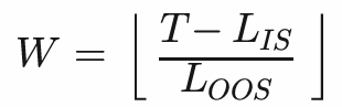
This follows from the rolling offset: the first IS window starts at index 0, and each step shifts by oos_length bars. The result array is sized to hold that many records before the loop begins.
Inside the loop, BuildWFEResults constructs each window's four boundary indices from the iteration counter. The IS window always starts at w multiplied by oos_length, placing the first window at the beginning of the array and each subsequent one one OOS-length step further along. The OOS window begins immediately after the IS window ends. A defensive break fires if the computed OOS end index would reach or exceed the array boundary, protecting against the off-by-one rounding that can occur on the final iteration.
For each window, ComputeSharpe is called twice — once for the IS slice and once for the OOS slice. If either call returns EMPTY_VALUE, the window record is marked invalid with all numeric fields zeroed and both flags set false, and the loop moves to the next window without incrementing the valid count. When both Sharpe values are usable, they are stored in the record, ComputeWFE produces the efficiency score, and the score is compared against the threshold to determine the pass flag. The valid count rises by one, and the loop continues until all windows are processed.
Aggregating the Distribution
ComputeWFEStatistics reduces the array of per-window records to six summary values written into reference parameters: the mean WFE, sample standard deviation, minimum, maximum, pass count, and fail count.
//+------------------------------------------------------------------+
//| Aggregate statistics across all valid WFE records                |
//+------------------------------------------------------------------+
void ComputeWFEStatistics(const WFERecord &results[],
                          int             num_windows,
                          double          &mean_wfe,
                          double          &stddev_wfe,
                          double          &min_wfe,
                          double          &max_wfe,
                          int             &pass_count,
                          int             &fail_count)
  {
//--- Initialize output parameters to safe states
   mean_wfe   = 0.0;
   stddev_wfe = 0.0;
   min_wfe    = DBL_MAX;
   max_wfe    = -DBL_MAX;
   pass_count = 0;
   fail_count = 0;

   int valid_n = 0;

//--- First pass: Compute sum, min, max boundaries and pass/fail counts
   for(int i = 0; i < num_windows; i++)
     {
      if(!results[i].is_valid)
         continue;

      double wfe = results[i].wfe;
      mean_wfe += wfe;

      if(wfe < min_wfe)
         min_wfe = wfe;
      if(wfe > max_wfe)
         max_wfe = wfe;

      if(results[i].is_pass)
         pass_count++;
      else
         fail_count++;

      valid_n++;
     }

//--- Guard against an empty distribution dataset
   if(valid_n == 0)
     {
      mean_wfe = 0.0;
      min_wfe  = 0.0;
      max_wfe  = 0.0;
      return;
     }

   mean_wfe /= (double)valid_n;

//--- Second pass: Compute variance for Sample Standard Deviation
   double sq_sum = 0.0;
   for(int i = 0; i < num_windows; i++)
     {
      if(!results[i].is_valid)
         continue;
      double dev = results[i].wfe - mean_wfe;
      sq_sum += dev * dev;
     }

//--- Calculate final sample standard deviation if sample size permits
   stddev_wfe = (valid_n > 1) ? MathSqrt(sq_sum / (double)(valid_n - 1)) : 0.0;
  }
All accumulators are initialized before the first pass — the minimum to the largest representable double and the maximum to the smallest, so that the first valid WFE value encountered always replaces both. The first pass walks every record in the array, skips any marked invalid, and for each valid record adds its WFE to the running sum, updates the min and max if the value extends the current range, increments the appropriate pass or fail counter, and increments the valid record count. If no valid records exist at all, the function zeroes the min and max outputs and returns early, avoiding a division-by-zero when computing the mean.
Once the first pass is complete, the mean is finalized by dividing the accumulated sum by the valid record count. A second pass is then required to compute the standard deviation, because measuring how far each value deviates from the mean is only possible once the mean itself is known. The second pass accumulates the squared deviations, and ComputeWFEStatistics takes their square root after applying the Bessel correction. The same two-pass structure used in ComputeSharpe is deliberately mirrored here for the same reason: numerical stability when values are close together relative to the magnitude of the mean.
Section 4: Rendering the Histogram
The visual output is handled by WFE_Canvas.mqh, which uses MetaTrader 5's native CCanvas library to paint a histogram directly onto the chart as a bitmap label object. The renderer produces an 800×500 pixels canvas on a white background, showing every window as a vertical bar growing upward from the zero baseline for positive WFE scores or downward for negative ones. Pass bars are rendered in deep green, fail bars in crimson. A dashed amber threshold line marks the 0.50 robustness boundary, and a dark blue horizontal line marks the mean WFE across all windows.
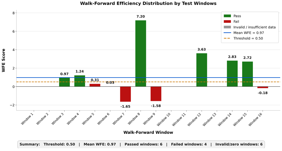
Figure 1: Walk-Forward Efficiency scores across 16 rolling windows, showing passing, failed, and invalid results relative to the 0.50 threshold.
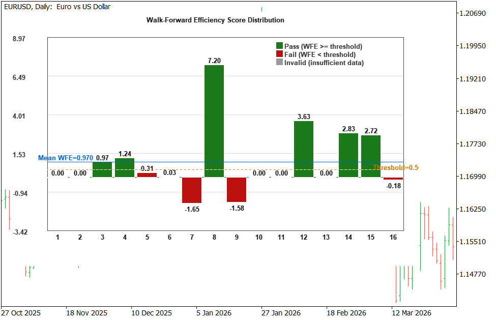
Figure 2: The same WFE histogram rendered as a bitmap label object directly on the EURUSD Daily chart inside MetaTrader 5. This contextual view demonstrates the technical implementation of the visualization within the trading terminal.
RenderWFEHistogram receives the complete array of scored windows, the threshold value, the precomputed mean WFE, and the chart ID, and writes everything to the canvas in a single rendering pass. The first action is to delete any existing canvas object with the same name before creating a fresh one, which ensures that re-running the script replaces the old histogram cleanly rather than layering a new one over it.
The coordinate transformation that maps a data value to a pixel Y position is:

This formula is used consistently for every element placed on the canvas — bar tips, gridlines, the threshold line, and the mean line — so that all elements share the same coordinate system and align precisely with each other. The Y-axis range is computed from the actual WFE data rather than a fixed scale, with 20% padding added above and below the data extremes so no bar tip touches the plot border. The threshold and mean values are explicitly included in the range scan, ensuring both reference lines always remain visible even when all WFE scores cluster far away from them.
Each bar is drawn as a filled rectangle extending from the zero pixel baseline to the pixel position corresponding to its WFE value. Positive values produce bars that grow upward; negative values produce bars that extend downward. A one-pixel border in the background color is drawn around each filled bar, which visually separates adjacent bars that would otherwise merge at their touching edges without requiring an explicit gap column in the layout. The threshold line is rendered as dashed by overwriting alternating four-pixel segments with the background color. CCanvas has no native horizontal dashed-line primitive. After all elements are painted, canvas.Update() flushes the pixel buffer to the display and ChartRedraw() triggers the terminal's repaint cycle.
Section 5: Empirical Validation
A scoring engine is only credible if it produces an honest verdict rather than the one its author expected. To test this, a Moving Average crossover Expert Advisor was built that runs in mean-reversion mode — fading each crossover rather than following it — and records its per-bar equity returns to CSV during a Strategy Tester backtest. Two configurations were scored with the WFE engine across EURUSD Daily data from 2021 through 2025.
Strategy A (optimized) had its parameters selected by the Strategy Tester optimizing the Sharpe ratio over the 2021–2023 in-sample period across a grid of FastMA periods from 3 to 19 (step 2), SlowMA periods from 20 to 60 (step 5), and MA methods SMA and EMA. The optimizer chose FastMA = 5, SlowMA = 25, SMA — the combination that maximized in-sample Sharpe on the calibration window. The full equity-return series for those parameters across all five years was then scored.
Strategy B (fixed) used FastMA = 10, SlowMA = 50, EMA — round, widely published values chosen on theoretical grounds with no optimization — scored across the identical five-year span.
Both runs produced 1,298 daily return bars and, with L_IS = 252 and L_OOS = 63, exactly 16 walk-forward windows:
W = ⌊ (1298 - 252) / 63 ⌋ = ⌊ 1046 / 63 ⌋ = 16
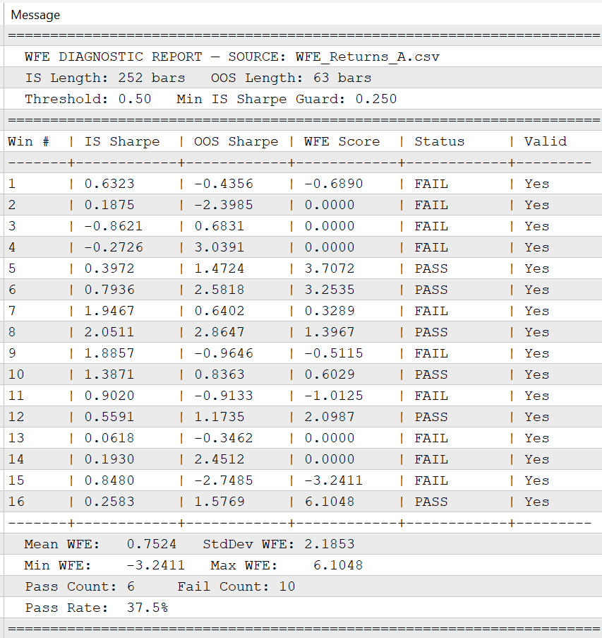
Figure 3: Experts tab output for Strategy A showing the full 16-window diagnostic table with IS Sharpe, OOS Sharpe, WFE Score, and Pass/Fail status for each window, followed by the aggregate statistics block.
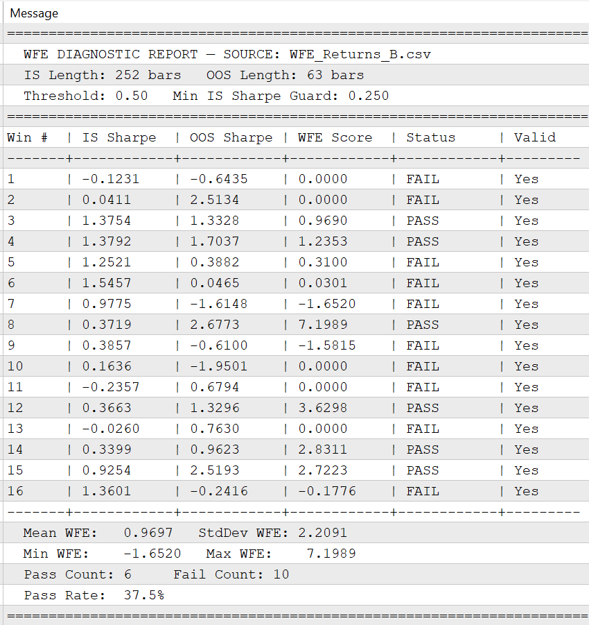
Figure 4: Experts tab output for Strategy B in the same format.
Strategy A Results (Optimized: FastMA=5, SlowMA=25, SMA)
| Window | IS Sharpe | OOS Sharpe | WFE | Status |
|---|---|---|---|---|
| 1 | 0.6323 | -0.4356 | -0.6890 | FAIL |
| 2 | 0.1875 | -2.3985 | 0.0000 | FAIL |
| 3 | -0.8621 | 0.6831 | 0.0000 | FAIL |
| 4 | -0.2726 | 3.0391 | 0.0000 | FAIL |
| 5 | 0.3972 | 1.4724 | 3.7072 | PASS |
| 6 | 0.7936 | 2.5818 | 3.2535 | PASS |
| 7 | 1.9467 | 0.6402 | 0.3289 | FAIL |
| 8 | 2.0511 | 2.8647 | 1.3967 | PASS |
| 9 | 1.8857 | -0.9646 | -0.5115 | FAIL |
| 10 | 1.3871 | 0.8363 | 0.6029 | PASS |
| 11 | 0.9020 | -0.9133 | -1.0125 | FAIL |
| 12 | 0.5591 | 1.1735 | 2.0987 | PASS |
| 13 | 0.0618 | -0.3462 | 0.0000 | FAIL |
| 14 | 0.1930 | 2.4512 | 0.0000 | FAIL |
| 15 | 0.8480 | -2.7485 | -3.2411 | FAIL |
| 16 | 0.2583 | 1.5769 | 6.1048 | PASS |
Mean WFE: 0.7524 | StdDev: 2.1853 | Min: -3.2411 | Max: 6.1048 | Pass rate: 37.5% (6/16)
Two engine behaviors visible in this table confirm the guards from Section 2 are working on real data. Window 2 has an IS Sharpe of 0.1875 — positive but below the 0.25 floor — and the near-zero guard correctly assigns it WFE = 0.0000 rather than dividing 0.1875 into -2.3985 to produce a large misleading negative number. Windows 3 and 4 have negative IS Sharpe values and the non-positive guard zeroes them regardless of their strong positive OOS performance. The engine refuses to credit forward performance that rests on a non-credible in-sample foundation.
Strategy B Results (Fixed: FastMA=10, SlowMA=50, EMA)
| Window | IS Sharpe | OOS Sharpe | WFE | Status |
|---|---|---|---|---|
| 1 | -0.1231 | -0.6435 | 0.0000 | FAIL |
| 2 | 0.0411 | 2.5134 | 0.0000 | FAIL |
| 3 | 1.3754 | 1.3328 | 0.9690 | PASS |
| 4 | 1.3792 | 1.7037 | 1.2353 | PASS |
| 5 | 1.2521 | 0.3882 | 0.3100 | FAIL |
| 6 | 1.5457 | 0.0465 | 0.0301 | FAIL |
| 7 | 0.9775 | -1.6148 | -1.6520 | FAIL |
| 8 | 0.3719 | 2.6773 | 7.1989 | PASS |
| 9 | 0.3857 | -0.6100 | -1.5815 | FAIL |
| 10 | 0.1636 | -1.9501 | 0.0000 | FAIL |
| 11 | -0.2357 | 0.6794 | 0.0000 | FAIL |
| 12 | 0.3663 | 1.3296 | 3.6298 | PASS |
| 13 | -0.0260 | 0.7630 | 0.0000 | FAIL |
| 14 | 0.3399 | 0.9623 | 2.8311 | PASS |
| 15 | 0.9254 | 2.5193 | 2.7223 | PASS |
| 16 | 1.3601 | -0.2416 | -0.1776 | FAIL |
Mean WFE: 0.9697 | StdDev: 2.2091 | Min: -1.6520 | Max: 7.1989 | Pass rate: 37.5% (6/16)
What the Comparison Shows
| Metric | Strategy A (optimized) | Strategy B (fixed) |
|---|---|---|
| Mean WFE | 0.7524 | 0.9697 |
| Pass rate | 37.5% | 37.5% |
| Std deviation | 2.1853 | 2.2091 |
| Min WFE | -3.2411 | -1.6520 |
| Max WFE | 6.1048 | 7.1989 |
The finding is direct and worth stating plainly: parameter optimization did not improve walk-forward robustness on this dataset. The fixed strategy modestly outperformed the optimized one on mean WFE (0.9697 versus 0.7524), and both passed an identical 37.5% of windows. Strategy A's worse minimum (-3.24 versus -1.65) indicates that its forward failures, when they occurred, were somewhat more severe — the kind of brittle reversal associated with curve-fitting a specific market regime — though the effect here is mild rather than catastrophic.
This is not the dramatic collapse a textbook overfitting example would show, and presenting it as one would misrepresent the data. The honest interpretation is more useful: the WFE engine returned an unsentimental verdict. It did not reward the optimized strategy for its higher in-sample Sharpe ratios — several of which, in windows 7, 8, and 9, exceeded anything Strategy B produced — because those in-sample peaks did not transfer forward consistently. The tool measured what actually generalized, not what looked impressive in calibration, and it did so without bias toward the configuration the researcher invested more effort in. For a validation instrument, that neutrality is the property that matters.
A practical caveat bounds these specific numbers. With only 16 windows, each WFE score carries wide estimation uncertainty, and the particular IS/OOS regime split is partly a matter of where the 2021–2025 period happened to place its trends and ranges. The conclusion to draw is about the engine's behavior — it scores honestly and guards correctly against the division pathologies — not a general claim about optimization always failing to help.
Section 6: Operational Constraints
Three limitations govern how far these scores can be trusted.
The WFE score is sensitive to the ratio L_IS / L_OOS. At the configuration used here, 252 / 63 = 4, the IS window estimates Sharpe from a full trading year while each OOS window rests on only 63 bars, giving individual OOS Sharpe estimates a standard error near 1 / √63 ≈ 0.13. Individual window scores should therefore be read as noisy; the distribution's center and pass rate carry more signal than any single bar in the histogram.
The Sharpe ratio assumes return stationarity within each window, which financial series violate through volatility clustering and regime shifts. A strategy calibrated in a calm IS period will show Sharpe compression in a turbulent OOS period regardless of parameter quality, and the engine cannot separate this structural effect from genuine overfit without additional conditioning on realized volatility. The negative-WFE windows in both tables are largely regime transitions of this kind rather than evidence of systematic strategy failure.
Finally, the minimum-data threshold is real. With L_IS = 252 and L_OOS = 63, a meaningful WFE distribution needs at least eight windows, implying a minimum dataset length of:
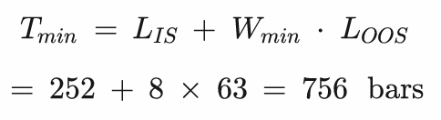
The five-year daily dataset used here clears that comfortably at 1,298 bars and 16 windows, but shorter histories will not support reliable scoring at these window sizes. If your available history is shorter, reducing L_OOS from 63 to 42 bars recovers more windows at the cost of noisier individual OOS Sharpe estimates.
Conclusion
The Walk-Forward Efficiency engine built in this article automates a measurement that is tedious to perform manually and easy to distort when done by eye. By expressing the relationship between in-sample and out-of-sample Sharpe as a single ratio per window, accumulating those ratios into a scored distribution, and rendering the result as a color-coded histogram, it converts the abstract concept of parameter robustness into a concrete, repeatable audit step that can be run on any strategy whose equity returns can be captured as a time series.
The empirical run produced a result that the engine had no reason to favor either way. The optimizer selected FastMA = 5, SlowMA = 25, SMA as its best configuration on the 2021–2023 in-sample period, and the fixed 10/50 EMA configuration outperformed it modestly on mean walk-forward efficiency across the full five-year span (0.9697 versus 0.7524), while both passed only 37.5% of their windows. The engine did not reward the optimized strategy for looking better in calibration. It measured what transferred forward, and reported it.
That is what a validation instrument should do. The three boundary conditions built into ComputeWFE — the non-positive guard, the near-zero guard, and the double-negative trap prevention — are not edge-case formalities. In the actual data, several windows triggered both guards and would have produced severely distorted scores without these protections. The guards fired silently and correctly on real data without any special handling by the caller.
For practitioners extending this work, the engine is indifferent to the source of the return series. Any strategy that can write a CSV of per-bar equity returns — whether a moving average crossover, a neural network signal, or an order-flow model — can be evaluated through this same pipeline. The IS and OOS window lengths, the robustness threshold, and the minimum IS Sharpe floor are all runtime inputs, making the engine adaptable to any timeframe and any definition of sufficient in-sample signal the practitioner wishes to impose.
Programs used in the article:
| # | Name | Type | Description |
|---|---|---|---|
| 1 | WFE_Engine.mqh | Include File | Core computation library containing the WFERecord struct, ENUM_TRADE_FREQUENCY, ComputeSharpe, ComputeWFE, BuildWFEResults, and ComputeWFEStatistics |
| 2 | WFE_Canvas.mqh | Include File | CCanvas histogram renderer covering background fill, gridlines, per-window bars, threshold and mean reference lines, legend, and pixel buffer flush |
| 3 | WFE_CSV_Reader.mqh | Include File | CSV reader that loads an EA-generated return series from the common files folder into a double array for engine consumption |
| 4 | WFE_Script_CSV.mq5 | Script | Executable script that wires the CSV reader, engine, and canvas together, prints the diagnostic table to the terminal log, and renders the histogram |
| 5 | MA_Crossover_EA.mq5 | Demo EA | Demo Expert Advisor that supports both mean-reversion and trend-following mode via a single input switch and writes per-bar equity returns to CSV on deinitialization |
| 6 | WFE.zip | Zip Archive | Zip archive containing all the attached files and their paths relative to the terminal's root folder. |
Warning: All rights to these materials are reserved by MetaQuotes Ltd. Copying or reprinting of these materials in whole or in part is prohibited.
This article was written by a user of the site and reflects their personal views. MetaQuotes Ltd is not responsible for the accuracy of the information presented, nor for any consequences resulting from the use of the solutions, strategies or recommendations described.

 MQL5 Trading Tools (Part 39): Adding a Pinned-Tools Ribbon for Quick Access to Favorite Tools
 Building a Broker-Agnostic Symbol Resolution Layer in MQL5
 MQL5 Bootstrap (II): Essential Validators for Robust Trading Systems
 Persistent Homology in MQL5: The Reduction Algorithm and the Persistence Diagram

- Free trading apps
- Over 8,000 signals for copying
- Economic news for exploring financial markets
You agree to website policy and terms of use