Foundation Models for Trading (Part I): Porting Kronos to Native MQL5

Introduction

A foundation model is a large neural network pretrained on vast data. It can be applied to many downstream tasks without retraining from scratch each time. Language models are the famous example, but the same idea has reached financial time-series modeling. Kronos is one such model. It is a transformer pretrained on millions of candlestick sequences. Given a window of recent bars, it forecasts the next bars (open, high, low, close, volume, and amount).

The interesting question for us is not whether such a model exists, but whether we can run it where our trading actually happens, inside MetaTrader 5, with no Python process in the loop at runtime. In this series we do exactly that. We take Kronos-small and its tokenizer and reimplement the entire forward pass by hand in native MQL5, using the platform's built-in matrix and vector types. Python is used only once, offline, to export the trained weights to flat binary files. After that, the terminal does all of the work on its own.

This first part covers the front half of the pipeline. It shows how weights move from PyTorch into MQL5, how raw candles are normalized and tokenized, and how a transformer block is assembled from primitive matrix operations. We finish by proving the port is correct against the original model, bit-for-bit, because everything that follows depends on that trust. The predictor, the autoregressive generation loop, and an honest evaluation of whether the forecast is worth anything come in later parts.

We will cover:

1. What a Foundation Model for Candlesticks Is
2. The Kronos Architecture
3. Why Not Just Use ONNX?
4. From PyTorch to .bin: The Offline Weight Bridge
5. Preprocessing: Z-Score Normalization and Timestamps
6. Binary Spherical Quantization: Candles to Tokens
7. Building the Transformer Block in MQL5 Matrix Ops
8. Proving It Is Correct: Golden-Reference Verification
9. Conclusion

What a Foundation Model for Candlesticks Is

Kronos treats a candlestick chart the way a language model treats text. A sentence is a sequence of tokens drawn from a fixed vocabulary. Kronos turns a sequence of candles into a sequence of discrete tokens drawn from its own learned vocabulary, then predicts the next token the way a language model predicts the next word. To generate a forecast, it samples tokens one at a time and converts them back into candles.

That design splits the model into two cooperating networks. The first is the tokenizer, an autoencoder that learns to compress a bar of six features into a pair of small integer tokens and to reconstruct the bar from those tokens. The second is the predictor, a decoder-only transformer that, given the token history, predicts the next pair of tokens. The two halves are trained separately and used together: encode the context window into tokens, let the predictor extend the token sequence, decode the new tokens back into candles.

The specific weights we port are Kronos-Tokenizer-base and Kronos-small, the smallest released pair. Even "small" here means a 512-dimensional, 8-layer transformer, so the forward pass is real work. Everything in this part concerns the tokenizer's encoder and the shared transformer machinery; the predictor and the decoder arrive in Part 2.

Fig. 1. The Kronos pipeline

From Fig. 1 we can see the shape of the whole system and where this article sits within it. The left half, raw candles becoming tokens, is what we build and verify here. The right half, tokens becoming a forecast, is Part 2.

The Kronos Architecture

Before porting anything, we need a clear picture of the model we are reproducing. Kronos has two parts that are trained separately and run together, and the whole design is captured in one diagram.

Fig. 2. The Kronos architecture. 

The tokenizer (left of Fig. 2). This is an autoencoder with a quantization bottleneck. The encoder embeds a bar's six features to model width and passes them through a stack of transformer blocks. BSQ then reduces each bar to a 20-bit code, split into a 10-bit coarse subtoken and a 10-bit fine subtoken, the s1 and s2 we met earlier. The decoder is a mirror stack that takes the code back to six features. The coarse subtoken carries the broad shape of the bar; the fine subtoken refines it. This is what makes the token space hierarchical, and it is the key to how the predictor generates.

The predictor (right of Fig. 2). This is a decoder-only causal transformer over the token history, the same family as a text language model. At each step it must produce a full token, both subtokens. It generates the coarse subtoken first from the transformer's output, then a small cross-attention head produces the fine subtoken conditioned on the coarse one just chosen. That ordering, coarse then fine, is why the hierarchy matters: the fine subtoken is never predicted blind, it always sees the coarse decision. We build this half in Part 2.

The two networks have different sizes, and getting these numbers exactly right is half the battle of a faithful port:

Hyperparameter	Tokenizer (base)	Predictor (small)
Model width (d_model)	256	512
Attention heads	4 (head_dim 64)	8 (head_dim 64)
Transformer blocks	3 (from a configured 4, the n-1 quirk)	8 (full count)
Feed-forward width	512	1024
Token vocabulary	2 x 1024 (s1, s2)	2 x 1024 (s1, s2)

The mathematics inside each block is modern but compact. Five operations define almost everything Kronos computes, and stating them now makes the code in the later sections read as a direct translation rather than a surprise.

RMSNorm. Normalization is root-mean-square only, with no mean subtraction and no bias, scaled by a learned per-feature weight.

RMSNorm(x) = x / sqrt(mean(x^2) + eps) * w

Here the mean of the squares is taken across the feature dimension of a single row, and w is the learned weight vector.

Rotary position embedding (RoPE). Position is encoded by rotating pairs of dimensions by an angle that grows with position, rather than by adding a position vector.

RoPE(x, t) = x * cos(t * theta) + rotate_half(x) * sin(t * theta),  theta_k = base^(-2k / hd)

The angle depends on the position t and the dimension index k; base is 10000 and hd is the head dimension. rotate_half swaps and negates the two halves of the vector.

SwiGLU feed-forward. The feed-forward network is gated: one projection is passed through a SiLU activation and multiplies a second projection elementwise, before a third projection restores model width. All three are bias-free.

SwiGLU(x) = W2 * ( SiLU(W1 * x) (.) (W3 * x) ),  SiLU(z) = z * sigmoid(z)

The symbol (.) denotes elementwise multiplication, the gate.

Scaled dot-product attention. Each query scores every key it is allowed to see, the scores are scaled and softmaxed, and the result weights the values.

Attention(Q, K, V) = softmax( Q * K^T / sqrt(hd) ) * V

In the encoder this is causal: a query at position i may only attend to keys at positions up to i, which preserves time order. In the predictor's cross-attention head it is non-causal, a point that causes real trouble in Part 2.

Binary Spherical Quantization. The quantizer's only effect on the token index is the sign of each latent coordinate.

bit_i = 1 if z_i > 0 else 0,  s1 = sum_(i<10) bit_i * 2^i,  s2 = sum_(i<10) bit_(10+i) * 2^i

We return to why only the sign survives, and the shortcut it buys us, in the tokenization section below.

Why Not Just Use ONNX?

MetaTrader 5 has native ONNX support, so the obvious question is why we hand-port the model at all instead of exporting it to ONNX and calling it from MQL5. It is the right question to ask, and the answer is specific to how this model runs.

ONNX represents a model as a static computation graph: a fixed sequence of tensor operations, tensors in, tensors out. That is an excellent fit for a single feed-forward network, such as one classifier or one regressor evaluated once per call. Kronos inference does not fit that pattern. It is an algorithm wrapped around several networks, and the algorithm is most of the difficulty:

• Autoregressive, with data-dependent control flow. The forecast is generated one token at a time in a loop, and the loop branches on its own state, a grow phase while the context is still filling and a slide phase once it reaches the maximum length. A static graph has no place to put that branch.
• A stateful cache that changes shape every step. Efficient generation keeps a key/value cache that grows by one row per step. Its shape is not fixed, which is precisely what a static graph cannot express.
• Sampling inside the loop. Each step draws tokens by multinomial sampling with temperature, top-k, and top-p filtering. This is stochastic control logic, not a tensor op.
• Discrete tokens between models. The encoder's output is quantized to integer tokens by a sign operation, the predictor consumes integer tokens and emits integer tokens, and only then does the decoder run. Three models with discrete, integer hand-offs are not one graph.
• A hierarchical dependency within each step. The fine subtoken is predicted only after the coarse subtoken for that same step has been sampled, an in-loop dependency between two sub-networks.

You could export each network to ONNX (encoder, predictor transformer, decoder). However, you would still have to implement in MQL5 the autoregressive loop, cache management, sampling, branching, token hand-offs, and the cross-attention ordering. That glue is the inference, and it is exactly where correctness is won or lost. Once it is written, the remaining matrix multiplies are the easy part, and doing them natively too keeps the whole pipeline in one place, one language, and one set of numbers we can verify end to end. That is why we port.

Note: For a single static network, ONNX in MQL5 is the right tool and far less work. The native port earns its keep specifically because Kronos inference is a dynamic, stateful, multi-model algorithm.

From PyTorch to .bin: The Offline Weight Bridge

Before MQL5 can run anything, the trained parameters have to leave PyTorch. There is no shared model format between the two worlds, so we use the simplest possible bridge: dump every tensor to a flat little-endian float32 file, and read those files back in MQL5 with FileReadArray. This happens once, offline, on a machine with PyTorch installed. At runtime the terminal never sees Python.

We start by cloning the official GitHub repository of Kronos:

git clone https://github.com/shiyu-coder/Kronos kronos-git

The exporter walks every parameter and buffer of each model and writes one .bin per tensor, alongside a manifest recording the original PyTorch name, the on-disk filename, and the shape. The core of export_kronos_weights.py is small:

# export_kronos_weights.py
def dump_module(mod, outdir, label):
    os.makedirs(outdir, exist_ok=True)
    manifest = {"label": label, "tensors": {}}
    tensors = list(mod.named_parameters()) + list(mod.named_buffers())
    total = 0
    print(f"\n=== {label} : {len(tensors)} tensors ===")
    for name, t in tensors:
        arr = np.ascontiguousarray(t.detach().cpu().float().numpy().astype(np.float32))
        fn = safe_name(name) + ".bin"
        arr.tofile(os.path.join(outdir, fn))
        manifest["tensors"][name] = {
            "file": fn,
            "shape": list(arr.shape),
            "dtype": "float32",
            "count": int(arr.size),
        }
        total += int(arr.size)
        print(f"  {name:55s} shape={tuple(arr.shape)}")
    manifest["total_params"] = total
    with open(os.path.join(outdir, "manifest.json"), "w") as f:
        json.dump(manifest, f, indent=2)
    print(f"  -> {total:,} values, manifest at {os.path.join(outdir, 'manifest.json')}")
    return manifest

The named_parameters() and named_buffers() calls together cover the learnable weights and the non-learnable state (such as normalization buffers), so nothing is missed. The PyTorch names contain dots and slashes that are awkward as filenames, so safe_name maps every non-alphanumeric character to an underscore. That mapping is recorded in the manifest, which becomes the contract the MQL5 loaders read against.

This detail prevents confusion later, so it is worth stating plainly. PyTorch stores a linear layer's weight with shape [out, in]: the matrix that computes y = x W^T + b is kept already transposed relative to the multiplication you write. Our .bin file is that raw [out, in] array, row-major. When we load it in MQL5 we will store it pre-transposed as [in, out], which lets the linear layer become a single matrix multiply with no per-call transpose. We return to why that matters for performance in Part 2; for now, just note that the file holds the PyTorch weight exactly as PyTorch holds it.

Fig. 3. The exported tokenizer and predictor weight folders with their manifest, placed under the terminal's MQL5\Files sandbox

The exported folders are copied under the terminal's MQL5\Files sandbox, because FileReadArray reads only from there. Fig. 3 shows the layout: one folder per model, a manifest, and a flat pile of .bin files named after their tensors.

Preprocessing: Z-Score Normalization and Timestamps

Kronos does not see raw prices. Each context window is normalized per feature before it ever reaches the model, and the same statistics are kept so the forecast can be returned to real price units afterward. The normalization is a plain z-score over the lookback window: subtract the column mean, divide by the column standard deviation, then clip to a fixed range to tame outliers.

Two choices here must match the reference exactly or the tokens drift. The standard deviation uses the population form, dividing by the row count, to match NumPy's default ddof=0. And a small eps is added to the denominator for stability. Here is KronosNormalize in full:

//+------------------------------------------------------------------+
//| Per-column z-score over the lookback rows, then clip.            |
//| raw[L][6] in feature order open,high,low,close,volume,amount.    |
//| mean/std are kept for the inverse transform. Population std      |
//| (divide by L) to match numpy ddof=0.                             |
//+------------------------------------------------------------------+
void KronosNormalize(const matrix &raw, matrix &norm, vector &mean, vector &stdv)
  {
   ulong L = raw.Rows();
   ulong F = raw.Cols();
   mean = vector::Zeros(F);
   stdv = vector::Zeros(F);
//--- per-column mean
   for(ulong j = 0; j < F; j++)
     {
      double s = 0.0;
      for(ulong i = 0; i < L; i++)
         s += raw[i][j];
      mean[j] = s / (double)L;
     }
//--- per-column population std (ddof = 0, matches numpy)
   for(ulong j = 0; j < F; j++)
     {
      double s = 0.0;
      for(ulong i = 0; i < L; i++)
        {
         double d = raw[i][j] - mean[j];
         s += d * d;
        }
      stdv[j] = MathSqrt(s / (double)L);
     }
//--- z-score, then clip to +/-KR_CLIP
   norm = matrix::Zeros(L, F);
   for(ulong j = 0; j < F; j++)
     {
      double denom = stdv[j] + KR_EPS;
      for(ulong i = 0; i < L; i++)
        {
         double v = (raw[i][j] - mean[j]) / denom;
         if(v >  KR_CLIP)
            v =  KR_CLIP;
         if(v < -KR_CLIP)
            v = -KR_CLIP;
         norm[i][j] = v;
        }
     }
  }

The six features are open, high, low, close, volume, amount, in that order. The clip is at plus or minus five standard deviations. Because the mean and standard deviation vectors are returned to the caller, the inverse transform that turns a normalized forecast back into prices is the same arithmetic in reverse, using exactly the statistics of the window the forecast was conditioned on.

Kronos also consumes timestamp features for every bar: minute, hour, weekday, day of month, and month. These feed learned temporal embeddings in the predictor. Most of those fields are trivial to fill, but one carries a genuine trap. The model was trained with pandas, whose weekday convention numbers Monday as 0 through Sunday as 6. MQL5's MqlDateTime numbers the week starting at Sunday as 0. If you pass the platform's value straight through, every weekday is wrong, and the temporal embedding the model receives is silently corrupted. The fix is a one-line remap:

//+------------------------------------------------------------------+
//| Timestamp features for one bar: [minute,hour,weekday,day,month]. |
//| Weekday is remapped from MQL5 (Sun=0..Sat=6) to the pandas       |
//| convention (Mon=0..Sun=6) the model was trained on.              |
//+------------------------------------------------------------------+
void KronosStamp(datetime t, int &out[])
  {
   MqlDateTime s;
   TimeToStruct(t, s);
   ArrayResize(out, 5);
   out[0] = s.min;
   out[1] = s.hour;
   out[2] = (s.day_of_week + 6) % 7;
   out[3] = s.day;
   out[4] = s.mon;
  }

The expression (day_of_week + 6) % 7 shifts Sunday from 0 to 6 and slides every other day down by one, reproducing the pandas numbering. It is a tiny change, but it is the kind of mismatch that produces a model which runs without error and forecasts nonsense.

Note: normalization statistics are computed per window, not globally. A forecast is only ever denormalized with the mean and standard deviation of the exact context window it was generated from. Mixing statistics across windows is a subtle way to corrupt the output.

Binary Spherical Quantization: Candles to Tokens

We met BSQ as a concept in the architecture section; now we implement it, because this is the part most readers will not have seen before and the implementation hides a useful shortcut. After the encoder's transformer blocks, a linear layer projects each bar to a 20-dimensional vector. BSQ quantizes that vector and the result is encoded as two 10-bit integers, the coarse token s1 and the fine token s2, each in the range 0 to 1023.

The full BSQ operation L2-normalizes the 20-dimensional vector onto a unit hypersphere, scales it, and quantizes each coordinate to the nearest of two values. But there is a shortcut that makes the MQL5 encoder both simpler and faster, and it is exact. The token index depends only on the sign of each of the 20 components. The L2-normalization and the scaling are strictly positive operations: they never change any coordinate's sign. So to compute the tokens, we can skip the normalization entirely and read the signs straight off the projected vector. Bit i is 1 when component i is positive, and the index is the usual sum of set bits times powers of two:

//+------------------------------------------------------------------+
//| BSQ encode: the s1/s2 indices depend only on the sign of each of |
//| the 20 z components (the L2-norm and scale before quantization   |
//| preserve sign). bit_i = 1 iff z_i > 0; index = sum bit_i * 2^i   |
//| (LSB-first).                                                     |
//+------------------------------------------------------------------+
void KronosBSQ_SignsToIndices(const double &z[], int &s1_id, int &s2_id)
  {
   s1_id = 0;
   s2_id = 0;
//--- s1: first KR_S1_BITS components (LSB-first)
   for(int i = 0; i < KR_S1_BITS; i++)
      if(z[i]              > 0.0)
         s1_id |= (1 << i);
//--- s2: next KR_S2_BITS components (LSB-first)
   for(int i = 0; i < KR_S2_BITS; i++)
      if(z[KR_S1_BITS + i] > 0.0)
         s2_id |= (1 << i);
  }

The first 10 components produce s1, the next 10 produce s2. The decoder needs the reverse: rebuild the 20-dimensional code from the two indices. Each bit becomes a bipolar value, plus or minus one over the square root of the dimension, which is the point on the hypersphere the quantizer would have produced:

//+------------------------------------------------------------------+
//| BSQ decode: rebuild the 20-dim bipolar code from the indices.    |
//| code_i = (bit_i * 2 - 1) / sqrt(20).                             |
//+------------------------------------------------------------------+
void KronosBSQ_IndicesToCode(int s1_id, int s2_id, double &code[])
  {
   ArrayResize(code, KR_CODEBOOK_DIM);
   double q = 1.0 / MathSqrt((double)KR_CODEBOOK_DIM);
//--- s1 bits -> first KR_S1_BITS code entries
   for(int i = 0; i < KR_S1_BITS; i++)
     {
      int b = (s1_id >> i) & 1;
      code[i]              = (b * 2 - 1) * q;
     }
//--- s2 bits -> next KR_S2_BITS code entries
   for(int i = 0; i < KR_S2_BITS; i++)
     {
      int b = (s2_id >> i) & 1;
      code[KR_S1_BITS + i] = (b * 2 - 1) * q;
     }
  }

Splitting the 20 bits into two 10-bit tokens is what makes Kronos hierarchical: s1 captures the coarse structure of the bar and s2 refines it, and the predictor learns to generate them in that order. We will use that hierarchy heavily in Part 2.

Fig. 4. Binary Spherical Quantization: the 20-dimensional latent vector is reduced to its per-coordinate signs, which pack into the s1 and s2 token ids

As Fig. 4 shows, the only information that survives quantization is which side of zero each coordinate falls on. There is one precision caveat worth keeping in mind: because the decision is a sign test, a component sitting extremely close to zero, within roughly a ten-millionth, could in principle flip between the MQL5 double computation and the reference float32. In practice that essentially never happens, and the verification in the last section confirms it: the tokens match exactly.

Building the Transformer Block in MQL5 Matrix Ops

Between embedding the candles and quantizing them sit the transformer blocks, and this is where most of the porting effort lives. Kronos uses a modern block: pre-normalization, RMSNorm instead of LayerNorm, rotary position embeddings, and a SwiGLU feed-forward. Every one of these has to be rebuilt from MQL5 matrix and vector operations. We will go through them in the order data flows.

The linear layer

Recall that we stored each weight pre-transposed as [in, out]. That decision pays off here: the linear layer is now a single matrix multiply with nothing else to do.

//+------------------------------------------------------------------+
//| Linear (PyTorch convention): y = x @ W^T. The weight is loaded   |
//| pre-transposed (KronosLoadMatrixT stores W as [in,out] == W^T),  |
//| so this is a plain MatMul with NO per-call transpose. Profiling  |
//| showed the old per-call W.Transpose() was ~60% of the forward    |
//| pass; the transpose now happens once at load. Math is identical. |
//+------------------------------------------------------------------+
matrix LinearT(const matrix &X, const matrix &W) { return X.MatMul(W); }

RMSNorm

Root-mean-square normalization scales each row by the reciprocal of the root mean of its squared entries, then multiplies by a learned per-feature weight. It has no mean-subtraction and no bias, which is what distinguishes it from LayerNorm.

//+------------------------------------------------------------------+
//| RMSNorm (row-wise): out = x / sqrt(mean(x^2) + eps) * weight.    |
//+------------------------------------------------------------------+
matrix RMSNorm(const matrix &X, const vector &w, double eps = KR_NORM_EPS)
  {
   ulong T = X.Rows(), D = X.Cols();
   matrix out = matrix::Zeros(T, D);
   for(ulong i = 0; i < T; i++)
     {
      double ms = 0.0;
      for(ulong j = 0; j < D; j++)
         ms += X[i][j] * X[i][j];
      ms /= (double)D;
      double scale = 1.0 / MathSqrt(ms + eps);
      for(ulong j = 0; j < D; j++)
         out[i][j] = X[i][j] * scale * w[j];
     }
   return out;
  }

SwiGLU

The feed-forward network is a gated variant. Two linear projections of the input are formed; one is passed through a SiLU activation and used to gate the other elementwise; a third projection brings the result back to model width. All three projections are bias-free.

//+------------------------------------------------------------------+
//| SiLU activation: x * sigmoid(x).                                 |
//+------------------------------------------------------------------+
double SiLU(double x) { return x / (1.0 + MathExp(-x)); }

//+------------------------------------------------------------------+
//| SwiGLU feed-forward: w2( SiLU(w1 x) * w3 x ), all bias-free.     |
//+------------------------------------------------------------------+
matrix SwiGLU(const matrix &X, const matrix &W1, const matrix &W3, const matrix &W2)
  {
   matrix H = LinearT(X, W1);
   matrix G = LinearT(X, W3);
   ulong T = H.Rows(), FF = H.Cols();
   matrix gated = matrix::Zeros(T, FF);
   for(ulong i = 0; i < T; i++)
      for(ulong j = 0; j < FF; j++)
         gated[i][j] = SiLU(H[i][j]) * G[i][j];
   return LinearT(gated, W2);
  }

Rotary position embeddings

RoPE encodes position by rotating pairs of dimensions by an angle proportional to the position. We precompute the cosine and sine tables once per sequence length, then apply them. Kronos builds its embedding by concatenating the frequency vector with itself, so the two halves of each row are duplicated, and the rotation pairs dimension k with dimension k + half.

//+------------------------------------------------------------------+
//| Build the RoPE cos/sin tables (T, hd). emb = cat(freqs, freqs),  |
//| so the two halves of each row are duplicated.                    |
//+------------------------------------------------------------------+
void RoPETables(ulong T, ulong hd, matrix &cosT, matrix &sinT)
  {
   ulong half = hd / 2;
   cosT = matrix::Zeros(T, hd);
   sinT = matrix::Zeros(T, hd);
   for(ulong t = 0; t < T; t++)
      for(ulong k = 0; k < half; k++)
        {
         double inv_freq = 1.0 / MathPow(KR_ROPE_BASE, (2.0 * (double)k) / (double)hd);
         double ang = (double)t * inv_freq;
         double c = MathCos(ang), s = MathSin(ang);
         cosT[t][k] = c;
         cosT[t][k + half] = c;
         sinT[t][k] = s;
         sinT[t][k + half] = s;
        }
  }

//+------------------------------------------------------------------+
//| Apply RoPE: out = x*cos + rotate_half(x)*sin, where              |
//| rotate_half(x) = cat(-x2, x1).                                   |
//+------------------------------------------------------------------+
matrix ApplyRoPE(const matrix &X, const matrix &cosT, const matrix &sinT)
  {
   ulong T = X.Rows(), hd = X.Cols(), half = hd / 2;
   matrix out = matrix::Zeros(T, hd);
   for(ulong t = 0; t < T; t++)
      for(ulong k = 0; k < hd; k++)
        {
         double rh = (k < half) ? -X[t][k + half] : X[t][k - half];
         out[t][k] = X[t][k] * cosT[t][k] + rh * sinT[t][k];
        }
   return out;
  }

Attention

Scaled dot-product attention for a single head computes query-key scores, scales them, applies a stable row-wise softmax, and weights the values. The causal flag masks each query so it can only attend to keys at or before its own position, which is what makes the encoder respect time order.

//+------------------------------------------------------------------+
//| Scaled dot-product attention for one head.                       |
//| Qh(Tq,hd), Kh(Tk,hd), Vh(Tk,hd). causal=true masks j>i and so    |
//| needs Tq==Tk. scores = Q.Kt * inv_sqrt -> stable row-softmax     |
//| -> weights . V. Returns Oh(Tq,hd).                               |
//+------------------------------------------------------------------+
matrix SDPA(const matrix &Qh, const matrix &Kh, const matrix &Vh, bool causal)
  {
   ulong Tq = Qh.Rows(), Tk = Kh.Rows(), hd = Qh.Cols();
   double inv_sqrt = 1.0 / MathSqrt((double)hd);
//--- scaled scores
   matrix scores = Qh.MatMul(Kh.Transpose());   // (Tq,Tk)
   scores *= inv_sqrt;
//--- row-wise softmax with optional causal mask
   for(ulong i = 0; i < Tq; i++)
     {
      //--- causal mask: query i attends to keys 0..i only
      ulong jmax = causal ? i : (Tk - 1);
      double smax = -DBL_MAX;
      for(ulong j = 0; j <= jmax; j++)
         if(scores[i][j] > smax)
            smax = scores[i][j];
      double denom = 0.0;
      for(ulong j = 0; j < Tk; j++)
        {
         if(causal && j > i)
           {
            scores[i][j] = 0.0;
            continue;
           }
         double e = MathExp(scores[i][j] - smax);
         scores[i][j] = e;
         denom += e;
        }
      double inv = 1.0 / denom;
      for(ulong j = 0; j < Tk; j++)
         scores[i][j] *= inv;   // masked entries already 0
     }
   return scores.MatMul(Vh);   // (Tq,hd)
  }

Multi-head attention wraps this: project the input to queries, keys, and values, split the columns into heads, rotate the queries and keys with RoPE, run attention per head, write the heads back, and apply the output projection. Notice the named locals Qs, Ks, Qh, and so on inside the head loop. That is not stylistic. It is the single most pervasive constraint of working with MQL5 matrices, and it deserves its own note.

Port trap: MQL5 matrix and vector objects are passed by reference only. You cannot pass a function's return value, a temporary, directly into a parameter that expects a matrix reference; the compiler rejects it. Every nested call's result must be assigned to a named local first, and that local passed onward. This is why the code reads matrix Qs = SliceCols(...); then ApplyRoPE(Qs, ...) rather than nesting the two. Method calls on a named object, such as X.MatMul(W), are fine.

//+------------------------------------------------------------------+
//| Causal multi-head self-attention with RoPE.                      |
//| q/k/v/out projections carry a bias.                              |
//+------------------------------------------------------------------+
matrix MHA(const matrix &X,
           const matrix &Wq, const vector &bq,
           const matrix &Wk, const vector &bk,
           const matrix &Wv, const vector &bv,
           const matrix &Wo, const vector &bo,
           int n_heads)
  {
   ulong T = X.Rows();
   ulong d_model = X.Cols();
   ulong hd = d_model / (ulong)n_heads;
//--- q/k/v projections (with bias)
   matrix Q = LinearT(X, Wq);
   AddRowBias(Q, bq);
   matrix K = LinearT(X, Wk);
   AddRowBias(K, bk);
   matrix V = LinearT(X, Wv);
   AddRowBias(V, bv);
//--- shared RoPE tables for all heads
   matrix cosT, sinT;
   RoPETables(T, hd, cosT, sinT);
   matrix ctx = matrix::Zeros(T, d_model);
//--- per-head causal attention
   for(int h = 0; h < n_heads; h++)
     {
      ulong c0 = (ulong)h * hd;
      matrix Qs = SliceCols(Q, c0, hd);   
      matrix Ks = SliceCols(K, c0, hd);
      matrix Qh = ApplyRoPE(Qs, cosT, sinT);
      matrix Kh = ApplyRoPE(Ks, cosT, sinT);
      matrix Vh = SliceCols(V, c0, hd);

      matrix Oh = SDPA(Qh, Kh, Vh, true);  
      WriteCols(ctx, Oh, c0);
     }
//--- output projection (with bias)
   matrix out = LinearT(ctx, Wo);
   AddRowBias(out, bo);
   return out;
  }

The block

With the pieces in place, the block itself is short. It is pre-norm: normalize, attend, and add the result back to the input as a residual; then normalize again, run the feed-forward, and add that back. The named locals here are the same reference constraint at work.

//+------------------------------------------------------------------+
//| Pre-norm block:                                                  |
//|   x += MHA(RMSNorm1(x)); x += SwiGLU(RMSNorm2(x)).               |
//+------------------------------------------------------------------+
matrix TransformerBlock(const matrix &X,
                        const vector &norm1_w,
                        const matrix &Wq, const vector &bq,
                        const matrix &Wk, const vector &bk,
                        const matrix &Wv, const vector &bv,
                        const matrix &Wo, const vector &bo,
                        int n_heads,
                        const vector &norm2_w,
                        const matrix &W1, const matrix &W3, const matrix &W2)
  {
//--- attention sub-block: x1 = x + MHA(RMSNorm1(x))
   matrix n1 = RMSNorm(X, norm1_w);                 // named locals: no temporaries by reference
   matrix a  = MHA(n1, Wq, bq, Wk, bk, Wv, bv, Wo, bo, n_heads);
   matrix x1 = X + a;
//--- feed-forward sub-block: out = x1 + SwiGLU(RMSNorm2(x1))
   matrix n2 = RMSNorm(x1, norm2_w);
   matrix f  = SwiGLU(n2, W1, W3, W2);
   return x1 + f;
  }

Fig. 5. Dataflow through the pre-norm block: each of the two residual branches normalizes its input, transforms it, and adds the result back to the stream

The encoder now reads as a clean chain. Embed the six features to model width, run the blocks, project to the 20-dimensional BSQ input, and read off the tokens. There is one more quirk hiding in the loop count, which we will meet in the code below.

   //+---------------------------------------------------------------+
   //| Encode a normalized window into hierarchical token ids.       |
   //|   x_norm        : (L, 6), preprocessed by KronosNormalize     |
   //|   s1_ids,s2_ids : output token ids, length L                  |
   //+---------------------------------------------------------------+
   bool              Encode(const matrix &x_norm, int &s1_ids[], int &s2_ids[])
     {
      if(x_norm.Cols() != KR_NFEAT)
        { PrintFormat("CKronosEncoder::Encode: expected %d feature cols, got %I64u", KR_NFEAT, x_norm.Cols()); return false; }

      //--- embed: 6 -> d_model
      matrix z = LinearT(x_norm, m_embedW);
      AddRowBias(z, m_embedB);
      //--- (n_enc_layers - 1) causal pre-norm blocks
      for(int b = 0; b < m_blocks; b++)
         z = TransformerBlock(z, m_n1[b],
                              m_Wq[b], m_bq[b], m_Wk[b], m_bk[b],
                              m_Wv[b], m_bv[b], m_Wo[b], m_bo[b],
                              m_heads, m_n2[b], m_W1[b], m_W3[b], m_W2[b]);
      //--- quant_embed: d_model -> 20 (this is the BSQ input z)
      matrix zq = LinearT(z, m_quantW);
      AddRowBias(zq, m_quantB);
      //--- BSQ: indices depend ONLY on sign of each of the 20 components, so the
      //--- L2-normalize + scale inside BinarySphericalQuantizer are skipped here
      ulong L = zq.Rows();
      ArrayResize(s1_ids, (int)L);
      ArrayResize(s2_ids, (int)L);
      double row[];
      ArrayResize(row, KR_CODEBOOK_DIM);
      for(ulong t = 0; t < L; t++)
        {
         for(int k = 0; k < KR_CODEBOOK_DIM; k++)
            row[k] = zq[t][k];
         int s1, s2;
         KronosBSQ_SignsToIndices(row, s1, s2);
         s1_ids[(int)t] = s1;
         s2_ids[(int)t] = s2;
        }
      return true;
     }

The loop runs m_blocks times, and m_blocks is set to n_enc_layers - 1. This is not a bug. The original tokenizer builds its block list with a range(n_layers - 1), so a configured count of four layers produces three blocks. It is an easy quirk to miss and an easy one to wrongly "correct." The predictor, as we will see in Part 2, does not share it and uses its full layer count, so the two must be treated differently.

Proving It Is Correct: Golden-Reference Verification

None of the above is worth anything if it does not match the original model, and "looks plausible" is not a standard. So the project is built with verification first: nothing is used before it is proven. But "proven" is not a single act. Verification here is a ladder with three rungs, and each rung catches a different class of mistake:

1. Weight-free unit tests of the individual primitives, which check that each operation obeys a property we can compute by hand, before a single trained weight is loaded.
2. A golden reference captured from the real PyTorch model on a frozen input, so there is a ground-truth number to compare against.
3. A per-stage harness that runs the MQL5 code on that same frozen input and compares its output to the golden reference.

We climb the ladder in that order. If a primitive is wrong, rung 1 catches it in isolation, with no weights and no reference to muddy the diagnosis. Only once the primitives are trusted do we load weights and compare the whole encoder against PyTorch.

Rung 1: weight-free self-tests. Before any weight is loaded, KronosSelfTests.mq5 checks each primitive against a property we can verify independently. These tests need no reference file, because the expected answer is known by construction. The clearest example is causal attention. If we feed it values 0, 1, 2, 3 down one column, zero the query and key projections so every query attends uniformly, and use an identity value projection, then a causal mask forces each output row to be the average of the values at or before its own position. Row 0 must equal V[0], row 1 the mean of the first two, and so on. That single test pins down the mask direction, the softmax normalization, and the value weighting all at once:

//+------------------------------------------------------------------+
//| Causal attention: each row is the mean of values up to that row. |
//+------------------------------------------------------------------+
void Test_Attention_Causal()
  {
   ulong d=4, T=4;
   matrix X = matrix::Zeros(T,d);
   for(ulong i=0;i<T;i++)
      X[i][0]=(double)i;
   matrix Z = matrix::Zeros(d,d), I = Identity(d);
   vector zb = vector::Zeros(d);
   matrix O = MHA(X, Z,zb, Z,zb, I,zb, I,zb, 1);
   CHECK(MathAbs(O[0][0]-0.0)<1e-12, "attn row0 = V[0]");
   CHECK(MathAbs(O[1][0]-0.5)<1e-12, "attn row1 = mean(V[0..1])");
   CHECK(MathAbs(O[3][0]-1.5)<1e-12, "attn row3 = mean(V[0..3])");
  }

#KronosSelfTests.mq5 output:

Kronos library self-test: 126 passed, 0 failed

ALL PASS -- weight-free units 1-3 verified.

The rest of rung 1 follows the same spirit. RoPE is checked to be the identity at position 0 and to preserve a vector's norm at every other position, both properties a correct rotation must have. RMSNorm is checked to produce unit root-mean-square output, the block wiring is checked to reduce to the identity when its projections are zeroed, and the BSQ index math is checked to round-trip an id to a code and back. None of these need a weight file, and together they mean that when the full encoder is finally assembled, every part it is built from is already known good.

Rung 2: capturing the golden reference. A property test proves a primitive is internally consistent, but it cannot prove the assembled encoder matches Kronos. For that we need a ground-truth number, produced by the real model. kronos_reference_capture.py is the counterpart to the weight exporter from earlier: where that script dumped the model's parameters, this one runs the model on a single frozen window and dumps its activations. It forces CPU and float32 for reproducibility, replicates Kronos's preprocessing exactly, then walks the model and saves each intermediate to a .bin file the MQL5 harnesses read verbatim. Here is the preprocessing, followed by the encoder call that produces the golden token ids:

    # --------------------------------------------- preprocessing (exact copy)
    x_mean = x_raw.mean(axis=0)                                  # (6,)
    x_std = x_raw.std(axis=0)                                    # (6,) population std, ddof=0
    x_norm = (x_raw - x_mean) / (x_std + args.eps)
    x_norm = np.clip(x_norm, -args.clip, args.clip).astype(np.float32)

    print("\nStage 0  preprocessing")
    save("x_raw", x_raw, np.float32)
    save("x_norm", x_norm, np.float32)
    save("x_mean", x_mean, np.float32)
    save("x_std", x_std, np.float32)
    save("x_stamp", x_stamp, np.float32)
    save("y_stamp", y_stamp, np.float32)

    xt = torch.from_numpy(x_norm)[None].to(device)              # (1, L, 6)
    xs = torch.from_numpy(x_stamp)[None].to(device)             # (1, L, 5)

    # ----------------------------------------------- Stage 1: tokenizer.encode
    print("\nStage 1  tokenizer.encode (half=True -> [s1_ids, s2_ids])")
    z_idx = tok.encode(xt, half=True)
    s1_ids = z_idx[0] if isinstance(z_idx, (list, tuple)) else z_idx
    s2_ids = z_idx[1] if isinstance(z_idx, (list, tuple)) else None
    save("s1_ids", s1_ids.cpu().numpy(), np.int32)
    if s2_ids is not None:
        save("s2_ids", s2_ids.cpu().numpy(), np.int32)

The x_std = x_raw.std(axis=0) line is the reference side of a match that has to be exact: NumPy's default is the population standard deviation (ddof=0), so the MQL5 KronosNormalize divides by the row count for the same reason. The save calls write each array both as a .npy for Python-side inspection and as a little-endian, row-major .bin the harness reads directly. The Stage 0 and Stage 1 labels are the first two steps of a longer ladder: the same script goes on to run decode_s1, decode_s2, and the tokenizer's decode, saving the predictor logits and the reconstruction as well.

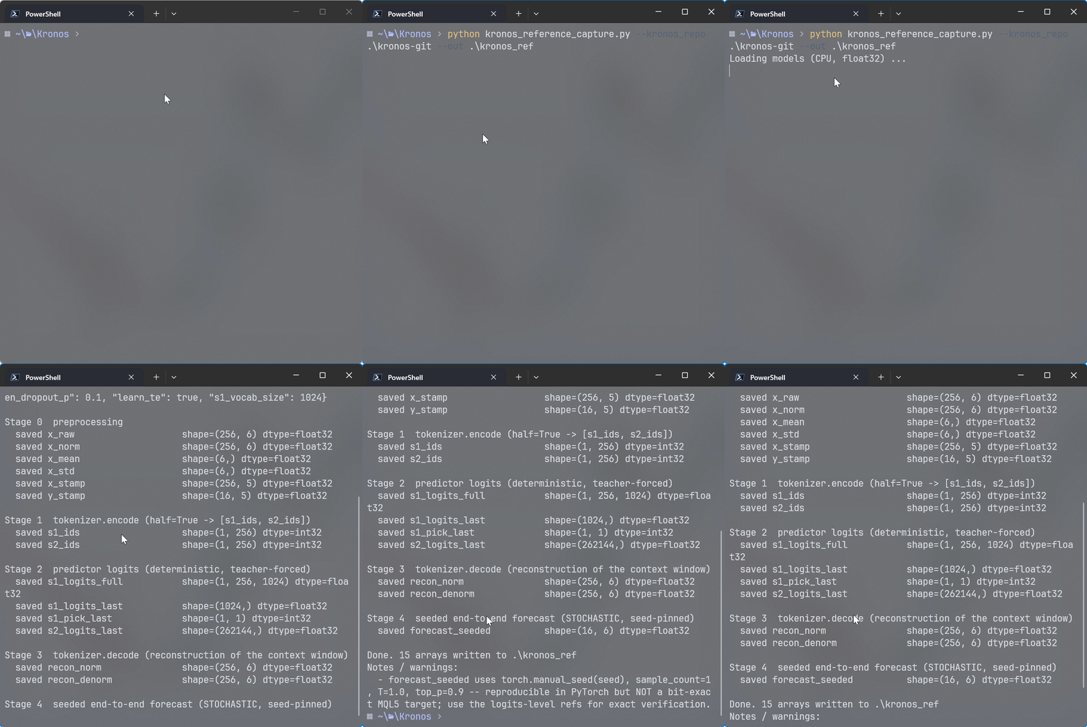
Fig. 6. The golden reference output. Forces CPU and float32 for reproducibility.

The whole capture is deliberately deterministic, with no sampling anywhere, so it is a single reproducible chain from the normalized input through the token ids to the logits and the reconstruction. One script captures the entire ladder in one run. Part 1 consumes only the first link, the token ids; the logits and the reconstruction are the golden references for the predictor and decoder we build in Part 2. The one discipline worth repeating is the reason CPU and float32 are forced above: a GPU run would not reproduce bit-for-bit, and the exactness of the comparison is the entire point.

Rung 3: the encoder harness. With a good reference in hand, the check itself is almost mechanical. KronosVerifyEncoder.mq5 loads the frozen x_norm, loads the golden s1_ids and s2_ids, builds and runs the MQL5 encoder on the exact same input, and compares. The body of the script reads top to bottom as those four steps:

   //--- 1) load the frozen normalized input window
   matrix x_norm;
   if(!LoadF32Matrix(InpRefDir + "x_norm.bin", (ulong)L, KR_NFEAT, x_norm))
     { Print("ABORT: could not load x_norm.bin"); return; }
   PrintFormat("Loaded x_norm: %I64u x %I64u", x_norm.Rows(), x_norm.Cols());

   //--- 2) load the golden token ids
   int ref_s1[], ref_s2[];
   if(!LoadI32Array(InpRefDir + "s1_ids.bin", L, ref_s1)) { Print("ABORT: s1_ids.bin"); return; }
   if(!LoadI32Array(InpRefDir + "s2_ids.bin", L, ref_s2)) { Print("ABORT: s2_ids.bin"); return; }

   //--- 3) build + load the encoder, run it
   CKronosEncoder enc;
   if(!enc.Init(KR_TOK_WEIGHT_DIR, KR_TOK_N_ENC_LAYERS, KR_TOK_D_MODEL, KR_TOK_N_HEADS, KR_TOK_FF_DIM))
     { Print("ABORT: encoder Init failed (weights/paths)"); return; }
   Print("Encoder weights loaded.");

   int s1[], s2[];
   if(!enc.Encode(x_norm, s1, s2))
     { Print("ABORT: Encode() failed"); return; }
   PrintFormat("Encode produced %d s1 ids, %d s2 ids", ArraySize(s1), ArraySize(s2));

   if(ArraySize(s1) != L || ArraySize(s2) != L)
     { PrintFormat("ABORT: length mismatch (got %d/%d, expected %d)", ArraySize(s1), ArraySize(s2), L); return; }

   //--- 4) exact integer comparison
   int first1, first2;
   int bad1 = CountMismatch(s1, ref_s1, L, first1);
   int bad2 = CountMismatch(s2, ref_s2, L, first2);

   PrintFormat("s1: %d / %d match  (mismatches: %d)", L - bad1, L, bad1);
   PrintFormat("s2: %d / %d match  (mismatches: %d)", L - bad2, L, bad2);

For token ids the bar is the highest possible: the tokens must be exactly equal, integer for integer, which is why CountMismatch tests a[i] != b[i] and not a tolerance. There is nothing to hide behind, because token ids are discrete; a single mismatched bit in one projected component would flip a token and show up here immediately. The result is a clean match: 256 of 256 on both token streams. When the counts come back short instead, the script goes on to print the first several offending positions with the MQL5 and reference values side by side, and the usual culprits are the transpose convention, the RoPE layout, or the block count, exactly the traps this article has been calling out.

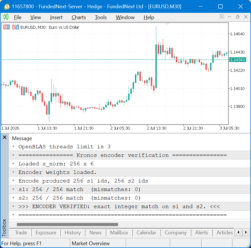
Fig. 7. The encoder verification harness reporting an exact integer match against the PyTorch reference on both token streams

This is also the moment the BSQ sign-only shortcut is validated. If any projected component had landed close enough to zero to flip sign between double and float32, the token at that bar would differ and the count would drop below 256. It does not. The decoder and the predictor are checked the same way against their own references from the same capture, with small floating-point tolerances appropriate to their continuous outputs; those results belong to Part 2, where we build them. What matters here is the principle the whole ladder exists to enforce: nothing is built blind, and nothing downstream is trusted until its input is proven.

Conclusion

We have built and verified the front half of a native MQL5 port of Kronos. Starting from a trained PyTorch model, we exported every weight to flat binary, normalized and timestamped raw candles the way the model expects, reduced each bar to a pair of hierarchical tokens through Binary Spherical Quantization, and assembled the transformer block, RMSNorm, RoPE, SwiGLU, and causal attention, from primitive matrix operations. The encoder reproduces the reference tokens exactly.

• No Python at runtime. The only offline step is a one-time weight export; the terminal runs the model itself.
• BSQ has a free shortcut. Because quantization preserves sign, the tokens are just the per-coordinate signs of the projected latent, no normalization needed, and it is exact.
• The traps are real. The pandas weekday remap, the by-reference-only matrix passing, and the n - 1 block count are each the kind of mistake that runs without error and corrupts the output silently.
• Verification is the foundation. An exact 256-of-256 token match is what lets us build the rest of the pipeline on top with confidence.

In Part 2 we cross to the other side of the model: the decoder that turns tokens back into candles, the predictor that generates new tokens, the cross-attention quirk that took real debugging to get right, and the autoregressive loop that produces a multi-bar forecast, along with the performance work that makes it run in a reasonable time.

The programs presented in this article are intended for educational purposes only. They demonstrate a porting and verification methodology, not a trading recommendation. Whether the model's forecasts carry any usable edge is a separate question, evaluated honestly in a later part of this series. Past performance and model fidelity do not guarantee future results.

Getting the Source Code via MQL5 Algo Forge

All source files are attached to this article below, but the full repository is also available on MQL5 Algo Forge, the community's Git-based platform for sharing and collaborating on trading projects. 

File name	Description
MQL5\Include\Kronos\KronosTokenizerMath.mqh	Preprocessing (z-score normalize/denormalize), timestamp builder with the weekday remap, BSQ sign/index math, and the weight loaders
MQL5\Include\Kronos\KronosTransformerCore.mqh	Transformer primitives: LinearT, RMSNorm, SwiGLU, RoPE tables and application, SDPA, causal self-attention, and the pre-norm block
MQL5\Include\Kronos\KronosEncoder.mqh	CKronosEncoder: the tokenizer encode chain from normalized candles to hierarchical s1/s2 token ids
MQL5\Scripts\Kronos\KronosSelfTests.mq5	Weight-free unit self-tests for the transformer primitives (LinearT, RMSNorm, SwiGLU, RoPE, attention), rung 1 of the verification ladder
MQL5\Scripts\Kronos\KronosVerifyEncoder.mq5	Golden-reference harness that checks the encoder tokens against the PyTorch reference (exact integer match), rung 3 of the ladder
MQL5\Kronos_Python\export_kronos_weights.py	Offline, one-time weight exporter: dumps every tensor to little-endian float32 .bin plus a manifest
MQL5\Kronos_Python\kronos_reference_capture.py	Offline, one-time: freezes a fixed input and captures the PyTorch golden references every harness checks against, rung 2 of the ladder