Neural Networks in Trading: An Intelligent Forecast Pipeline (Time-MoE)

Introduction

Time series forecasting remains one of the key tasks upon which modern algorithmic trading is based. The accuracy of the model determines not only the success of a trading strategy, but also its ability to adapt to the ever-changing nature of the market. Most models were designed for a specific task and lost their robustness at the slightest change in the market environment. Recently, so-called foundation models have been developing rapidly. One such model was presented in the article "Time-MoE: Billion-Scale Time Series Foundation Models with Mixture of Experts".

Time-MoE is a next-generation decoder-only Transformer designed specifically for time series data. It is based on the principles of sparse learning, modularity, and forecasting at multiple scales. The framework's authors demonstrate how the scalability and flexibility of large models can be extended to the realm of time series without sacrificing computational efficiency. The model architecture they present supports arbitrary lengths of analyzed sequences and forecast horizons. At the same time, the model can process data streams in real time.

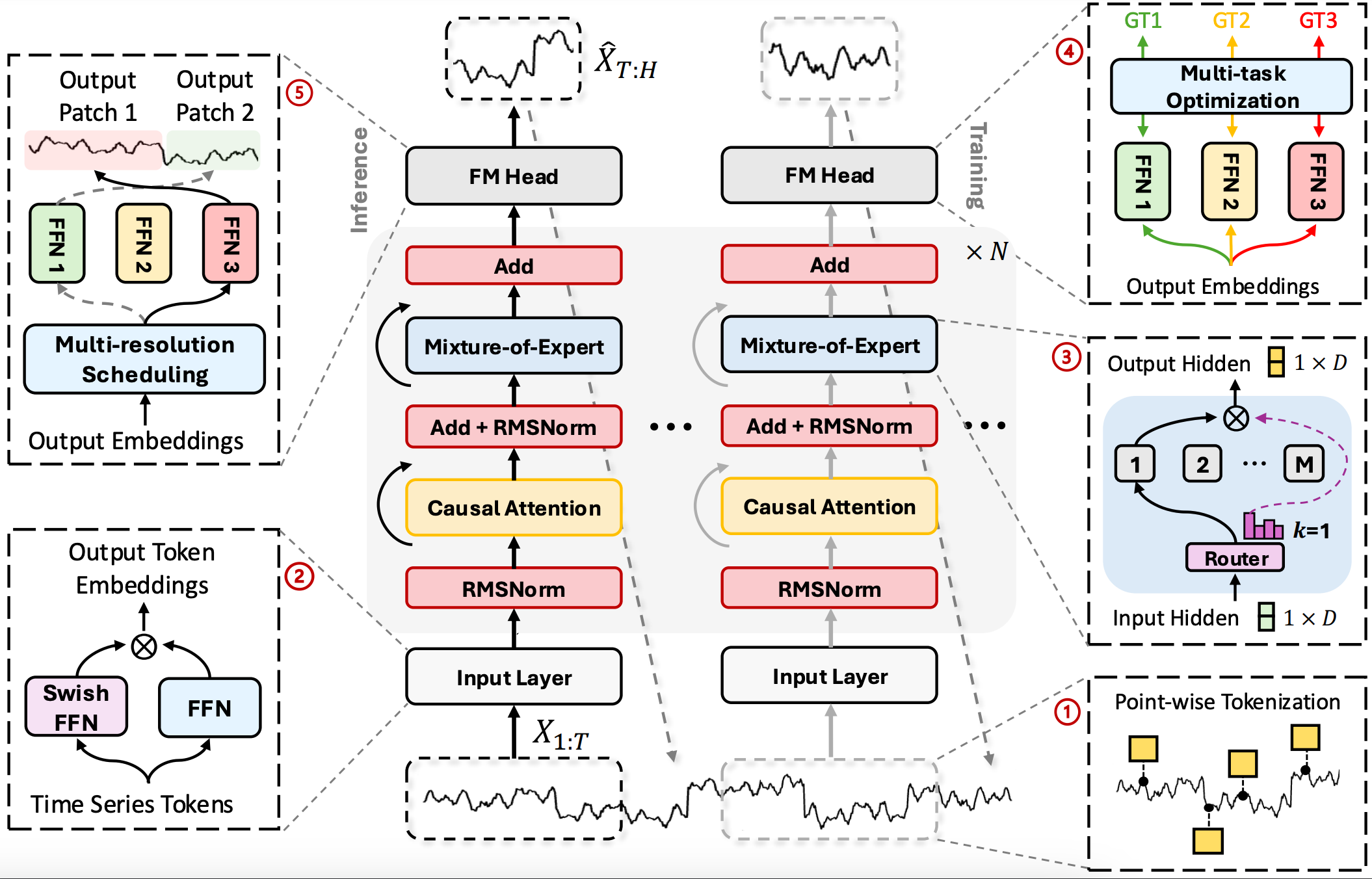
The first component of the architecture is point-wise tokenization of the time series (Point-Wise Tokenization). Unlike window-based or aggregated approaches, each time step here is converted into a separate token. This feature can be useful in high-frequency trading, where even a single tick can change the market picture. In the MQL5 environment, tokens can be formed from bars, ticks, and derived indicators, including volatility, volume, and signals from custom strategies.

After tokenization, the data are passed through an embedding layer with SwiGLU activation, which is a hybrid of Swish and a Gated Linear Unit. It allows for smoother and more robust representations of the analyzed information, which is particularly useful in the presence of market noise and unstable trends.

At the core of the model is a stack of N repeated blocks, each of which combines causal multi-head self-attention (Causal Multi-Head Self-Attention) and a sparse mixture of experts (Sparse MoE). Attention is directed strictly toward the past, which guarantees a proper chronology: the model has no access to future data and is therefore applicable in real market conditions. MoE adds scalability to the architecture: instead of activating all model parameters, a limited number of specialized submodels (experts) are selected for each token. Some learn to handle impulsive movements better, while others specialize in consolidation phases or range-bound markets. The adaptive mechanism determines how tokens are routed.

However, the model does not stop at the data processing stage. One of the key features of TIME-MOE is multiscale forecasting (Multiscale Forecasting). During training, the model is tasked with making predictions simultaneously across different forecast horizons. This is implemented through parallel output modules (heads), each of which is trained on its own target label: short-term, medium-term, or long-term. This architecture makes it possible to capture both market microdynamics and broader market behavior simultaneously. The model is capable of switching between them depending on the market context.

During inference, dynamic forecasting head selection (Dynamic Head Scheduling) comes into play. Depending on volatility, trend strength, or model confidence, different forecasting modules are activated. This adaptive approach makes Time-MoE particularly valuable in trading, where market behavior can change in an instant.

It is important to note that Time-MoE is optimized for training on large-scale time-series datasets. The framework's authors trained the model on Time-300B — the largest open dataset, containing more than 300 billion time-series data points from nine domains. This made it possible to achieve high model versatility, robustness to distribution shifts, and the ability to generalize to unseen tasks. At the same time, Time-MoE scales to 2.4 billion parameters while activating only a subset of them during inference, making it both high-performing and resource-efficient.

The Time-MoE Algorithm

Time-MoE is based on the idea of creating a unified, scalable model for time-series forecasting that can adapt to any conditions in the analyzed environment while keeping the load on computational resources manageable. The framework's algorithm begins with point-wise tokenization (Point-Wise Tokenization), where all important features of each step in the time series are captured. This approach ensures that no detail is lost during aggregation.

The transformation of raw tokens into an informative latent space is performed using a SwiGLU embedding.

where the matrices W and V are trained together with the model. Element-wise multiplication ⨂ amplifies significant features, and the combination of the Swish function and the gating mechanism (Gated Linear Unit) produces more expressive embeddings capable of encoding complex nonlinear dependencies.

After embedding, the tokens are fed into a stack of N identical Transformer blocks. Each block consists of three stages:

1. Normalization and causal attention: the input vectors h_{t,l-1} are first normalized and then analyzed by multi-head Self-Attention with a mask that prevents access to future values. The token turns its head back, looking over the entire history so far, but at the same time cannot look ahead, as if following a strict rule: current decisions are based solely on past experience.
   



where SA stands for Self-Attention with H heads, each of which analyzes the previous t-1 positions. This design allows the model to track important events in the history while preserving causal relationships.

2. A second normalization helps avoid overreacting to rare anomalies.



3. A sparse Mixture-of-Experts layer. Here, we route each historical window to a group of experts — a Mixture-of-Experts. The adaptive router decides which K experts out of N to activate. The shared (N+1)-th expert always participates via a sigmoid weighting function. Active experts process the data independently and return their forecasts. The final output of the block is summed with the input signal.

This structure enables dynamic specialization selection: during periods of high volatility, tokens are routed to experts trained to recognize impulsive movements, whereas in calmer periods they are routed to those that are better suited to handling trends or range-bound regimes. Top-K expert selection makes it possible to limit the number of active subnetworks while keeping the bulk of the parameters in a dormant state. This allows the model to be scaled up to billions of parameters while maintaining a constant inference budget.

When the token xT passes through all N layers, we obtain a contextual vector hT,L that contains the entire market history and its patterns. For Multi-Resolution Forecasting, P forecasts are generated from it for forecast horizons p1, …, pP using single-layer FFNs.

This architecture makes it possible to generate forecasts for different time spans simultaneously while preserving a unified hidden representation.

During training, the model faces the task of predicting multiple forecast horizons simultaneously: from near-term minute-by-minute fluctuations to longer-term trends unfolding over days and weeks. For each forecast, the framework's authors use Huber loss, which combines the smoothness of the quadratic component with the robustness of the linear part. For small errors, Huber loss behaves like the classical MSE, gently penalizing small deviations, while for large errors it gradually transitions to L1, reducing the impact of rare outliers and preventing gradient explosion. The model then aggregates the losses across all forecasting heads.

Thanks to this approach, the model learns to capture short-term impulsive movements and track long-term trends at the same time, while preserving forecast coherence at all levels.

However, the use of sparse experts (MoE) creates a risk of uneven workload distribution: some experts may become overloaded, while others may remain idle. To mitigate this effect, an auxiliary regularization term was added to measure the imbalance. The final training objective is the sum of the main and auxiliary components.

The end result is a unified, coordinated pipeline: from fine-grained tokenization to dynamic routing across experts, multi-level forecasting, and balanced training.

The authors' visualization of the Time-MoE framework is shown below.

Implementation in MQL5

Now that we have taken a detailed look at the theory and key aspects of the Time-MoE framework, it is time to move on to the practical part of our work and bring the theory to life in code. However, rather than trying to tackle the whole thing at once, we will break the entire system down into logical blocks. Following the flow of information, we will implement the framework step by step using MQL5. This phased, practice-oriented approach will not only make it easier to test and debug each module, but will also allow us to assemble them into a fully functional, responsive Time-MoE implementation ready for powerful and efficient operation in real-world market conditions.

According to the original concept proposed by the authors of Time-MoE, all input data passes through the point-wise tokenization module, which can be efficiently implemented using an existing convolutional layer. Essentially, each bar or tick is fed into a short 1D convolutional filter, and the result of the convolution is nothing more than an atomic token with a set of features. This technique gives us two important advantages: first, we preserve information about every point in time without the losses associated with aggregation; second, convolution immediately detects local patterns.

Next, the data are passed to the SwiGLU embedding, which we will work on next.

SwiGLU Embedding

After the tokens are generated, they are sent to the second stage — the SwiGLU embedding module, which transforms the raw features into expressive hidden-space vectors. The SwiGLU layer performs a dual transformation:

1. First, the token passes through a linear projection and the soft, smooth Swish function;
2. then through another projection and a selective Gated Linear Unit (GLU).

At the output, the two results are combined using element-wise multiplication.

Swish smooths the embedding, allowing the model to capture subtle signals, while GLU opens or closes individual vector components, highlighting truly important patterns.

In our implementation, the SwiGLU layer will be represented as the CNeuronSwiGLUOCL class, which inherits from the base neural layer object. Inside this class, we will create two special convolutional layers that perform a dual projection of the analyzed vector and output two versions of the signal. The structure of the new object is shown below.

class CNeuronSwiGLUOCL  :  public   CNeuronBaseOCL
  {
protected:
   CNeuronConvOCL    caProjections[2];
   //---
   virtual bool      feedForward(CNeuronBaseOCL *NeuronOCL)          override;
   virtual bool      updateInputWeights(CNeuronBaseOCL *NeuronOCL)   override;
   virtual bool      calcInputGradients(CNeuronBaseOCL *NeuronOCL)   override;

public:
                     CNeuronSwiGLUOCL(void) {};
                    ~CNeuronSwiGLUOCL(void) {};
   //---
   virtual bool      Init(uint numOutputs, uint myIndex, COpenCLMy *open_cl, uint window,
                          uint step, uint window_out, uint units_count, uint variables, 
                          ENUM_OPTIMIZATION optimization_type, uint batch);
   //---
   virtual int       Type(void) override const {   return defNeuronSwiGLUOCL; }
   //--- methods for working with files
   virtual bool      Save(int const file_handle)   override;
   virtual bool      Load(int const file_handle)   override;
   //---
   virtual void      SetOpenCL(COpenCLMy *obj)     override;
   //---
   virtual bool      WeightsUpdate(CNeuronBaseOCL *source, float tau) override;
  };

All internal objects of our new class are declared statically. Therefore, the constructor and destructor remain empty. Initializing all projections, convolution parameters, and the connection to the OpenCL context is handled by the Init method. It is in the parameters of this function that the user specifies the convolution window size, the stride, the number of filters, and a pointer to the OpenCL context. All this makes it possible to fully configure the layer before use.

bool CNeuronSwiGLUOCL::Init(uint numOutputs, uint myIndex, COpenCLMy *open_cl,
                            uint window, uint step, uint window_out, uint units_count,
                            uint variables, ENUM_OPTIMIZATION optimization_type, uint batch)
  {
   if(CNeuronBaseOCL::Init(numOutputs, myIndex, open_cl, units_count * window_out * variables,
                                                                    optimization_type, batch))
      return false;
   SetActivationFunction(None);

Inside the method, we delegate all basic setup upward — to the parent-class level, where basic validation and common interface setup are already implemented there. To do this, simply call the method of the same name in the parent class. This allows us to avoid duplicating low-level operations and to be confident in the reliability of the execution environment.

Here, we explicitly disable the activation function of our layer at the interface level, since all nonlinearities are implemented by internal objects.

Once the infrastructure details have been worked out, we move on to fine-tuning our layer. It is important to note here that both internal convolutional layers are designed to produce vectors of the same size — this is critically important. After all, only when the dimensions match can we correctly multiply them element by element. The only difference between them lies in the subsequent use of different activation functions.

Therefore, during the preparation phase, we initialize these layers in a loop, automatically assigning each one the same convolution window configuration, number of filters, and stride. This avoids code duplication and ensures that both projections always remain dimensionally consistent.

for(uint i = 0; i < caProjections.Size(); i++)
  {
   if(!caProjections[i].Init(0, i, OpenCL, window, step, window_out, units_count,
                                                variables, optimization, iBatch))
      return false;
  }

Once the dimensions and basic parameters have been verified, we configure a separate activation function for each layer so that the resulting embeddings exhibit a combination of smooth and selective features. This approach simplifies code maintenance and ensures a clear separation of roles within the SwiGLU layer.

   caProjections[0].SetActivationFunction(GELU);
   caProjections[1].SetActivationFunction(None);
//---
   return true;
  }

Now we can complete the initialization method of the SwiGLU layer by returning the boolean result of the operations to the calling program.

Once all the layer settings are complete, it is time to fire up the engine and run the data being analyzed through our two convolutional projections. Let's begin building the forward pass algorithm, which is implemented in the feedForward method.

bool CNeuronSwiGLUOCL::feedForward(CNeuronBaseOCL *NeuronOCL)
  {
   for(uint i = 0; i < caProjections.Size(); i++)
      if(!caProjections[i].FeedForward(NeuronOCL))
         return false;

As usual, in the parameters of this method, we receive a pointer to the input data object. This is precisely what we need to pass into both of our data projection layers. We perform this operation in a loop. Declaring an array of objects gives us this capability.

It is precisely because both layers produce tensors with the same dimensions that we can directly multiply them element by element, without worrying about mismatched dimensions. The result is a single output tensor, where each value is the product of the “opinions” of the Swish and GLU projections. This technique, based on cyclically passing a pointer to the data through the array of layers, keeps the code compact and makes it easy to scale the number of “voices” within the layer simply by changing the length of the array.

   if(!ElementMult(caProjections[0].getOutput(), caProjections[1].getOutput(), Output))
      return false;
//---
   return true;
  }

We store the obtained results in the layer’s output buffer and finish the method by returning a Boolean result to the calling program.

Once the forward pass through the SwiGLU layer is complete, it is time to trace where every drop of error went — and set up the backward pass. The idea is to distribute the gradient from the output level back to the input data, carefully passing it through both of our convolutional projectors. This process is implemented in the calcInputGradients method.

bool CNeuronSwiGLUOCL::calcInputGradients(CNeuronBaseOCL *NeuronOCL)
  {
   if(!NeuronOCL)
      return false;

In the method body, we obtain a pointer to the input data object. The same one we used during the forward pass. Only this time, we need to return the error gradient to it in proportion to the influence of the input data on the final result. Of course, a valid object is required for the data to be passed correctly. Therefore, before proceeding with further operations, we check whether the pointer we received is valid.

In our layer's external interfaces, we already have the difference between the current forecast and the target value. Next, because the vector dimensions match, we can easily isolate the portion of the error attributable to each internal filter.

if(!ElementMultGrad(caProjections[0].getOutput(), caProjections[0].getGradient(),
                    caProjections[1].getOutput(), caProjections[1].getGradient(),
                    Gradient, caProjections[0].Activation(), caProjections[1].Activation()
                   ))
   return false;

We send these two streams to the corresponding convolutional neurons. Because both layers maintain their own gradient buffers, each of them receives its own vector with the same dimensions as the input data.

After that, each internal convolutional object will independently propagate its portion of the error further. But this time, we cannot pass values to the input data object inside the loop. The problem is that each subsequent operation will overwrite the data, deleting what was previously saved. We, on the other hand, need to aggregate the values from all information flows. Therefore, we first pass the error gradients from the first projection layer.

if(!NeuronOCL.calcHiddenGradients(caProjections[0].AsObject()))
   return false;

Then, we store a pointer to the input data object's error gradient buffer in a local variable. Another free data buffer of the same size will take its place.

   CBufferFloat *temp = NeuronOCL.getGradient();
   if(!NeuronOCL.SetGradient(NeuronOCL.getPrevOutput(), false) ||
      !NeuronOCL.calcHiddenGradients(caProjections[1].AsObject()) ||
      !SumAndNormilize(temp, NeuronOCL.getGradient(), temp, 1, false, 0, 0, 0, 1) ||
      !NeuronOCL.SetGradient(temp, false)
     )
      return false;
//---
   return true;
  }

And now we can safely pass the data through the second information flow. Next, we sum the values obtained from the two projection layers. This approach ensures that every bit of error from different information flows is preserved and correctly aggregated, providing us with an accurate and stable weight update in the subsequent optimization step.

Finally, we restore the pointers to the data buffers to their original state and complete the method by returning the Boolean result of the operations to the calling program.

As usual, the backward pass algorithm is divided into two logical stages. We have already discussed the first stage — distribution of the error gradient — in detail. This is a key step that allows the error to be passed correctly from the layer output to the input data, while taking into account all the characteristics of the multi-branch information flow.

The second stage — parameter optimization, aimed at reducing the overall error — is beyond the scope of this article. Not because it is unimportant, but because its implementation is strictly encapsulated within each of the convolutional objects. This gives us an important advantage: the interface of our class is not overloaded with unnecessary details, but instead preserves architectural purity and modularity.

All the necessary steps for updating the weights have already been implemented within each projection layer. Therefore, to complete the entire optimization cycle, we simply need to call the corresponding methods of all internal objects in sequence. Thanks to this approach, the main class remains compact, and the logic for updating parameters is reliable and has been tested in isolation.

The complete source code for the CNeuronSwiGLUOCL class and all of its methods, including the forward pass and backward pass functions, is provided in the attachment and can be reviewed to gain a deeper understanding of all the internal mechanisms of its operation.

We have completed the implementation of the SwiGLU embedding component, and we can now confidently move on to the next stage — implementing the core part of the Time-MoE framework: the modified Transformer block. This step marks a new chapter in model development, as it is within the transformer block that a high-level understanding of the sequence is formed: the model learns to identify long-term dependencies, analyze context, and forecast the likely dynamics of future events.

Passing the transformed time series from the SwiGLU block to the Transformer module is not simply a transfer of data, but, in essence, a transfer of knowledge. Embeddings, compressed and rich with information about local patterns, now become the basis for in-depth analysis. However, the Transformer architecture in Time-MoE differs significantly from the classical implementation. The first thing that stands out is the absence of the familiar FeedForward block, which usually follows immediately after the attention mechanism in each layer.

Instead of the standard module, the authors proposed using what is known as a sparse mixture of experts (Sparse Mixture of Experts, or simply MoE). This architectural choice not only gives the model adaptive flexibility but also makes its training more meaningful and context-dependent. The main idea of MoE is to break down a single universal layer into a set of highly specialized submodules (experts), each of which is trained to process a specific type of input data. This approach allows each token in the input sequence to consult only those experts that are best suited to process its specific features, while leaving the others in standby mode.

The adaptive expert selection mechanism is implemented using a router — a separate submodule that, based on the token's initial representation, determines which experts will be involved. The original article highlights an important point: it uses sparse routing, in which each token is routed not to all experts at once, but only to a few (for example, two out of ten possible experts). This significantly reduces computational costs, making it possible to use MoE even on a large scale without placing a critical strain on resources.

This approach offers the model numerous advantages. First, it learns to distribute tasks among experts: some adapt to short-term price fluctuations, while others adapt to trending movements or volatility. Second, the model gains the ability to generalize knowledge: because different experts acquire different experience, it can model more complex interactions than in a traditional single-level architecture.

Thus, the use of Sparse Mixture of Experts in the Time-MoE transformer can be considered the framework’s central innovation. This is not just an architectural experiment — it is a fundamental rethinking of the approach to processing time series.

This brings us to the question: how can we put these architectural ideas into practice? After all, we are not just theorizing — we are building a working system step by step. Looking back at the previous stages of our research, we have already encountered the concept of Mixture of Experts (MoE) in the context of developing the DUET framework. At that time, we developed a very simple prototype that helped us better understand how routing and the aggregation of expert decisions work. However, it would be difficult to call that implementation truly sparse. Rather, it was an imitation of the selection mechanism: all the experts computed their outputs simultaneously, and then their results were simply multiplied by the corresponding masks.

From a mathematical standpoint, the final result looked plausible: the masks made it possible to zero out the outputs of unneeded experts, thereby forming a controllable superposition. However, from the standpoint of computational efficiency, we were, frankly, falling short. After all, in this case, each expert still carried out its full workload, regardless of whether its result would be used or not. Thus, the computational complexity grew linearly with the number of experts, which negated one of the key advantages of the MoE architecture—its ability to scale without exponential growth in cost.

This approach is, of course, acceptable for small models, where the number of experts and their dimensions are modest, and performance requirements are not so critical. However, in real-world scenarios — for example, when working with deep and wide transformers, where MoE is used in every other layer and the number of experts can reach into the tens — such a solution simply becomes unfeasible. The computational load quickly exceeds reasonable limits, especially if we want to use the model in real time — for example, for algorithmic trading in financial markets.

In addition, as the number of experts increases, the routing process itself becomes more complex. If we continue to use them all at once, we will inevitably run into GPU memory usage and a loss of performance in OpenCL. And this is where it becomes especially important to adhere to the philosophy of true sparsity: let only a small part of the network be active — but precisely the part that is needed right here and now. This approach not only conserves resources but also makes the model itself more adaptive and robust to noise.

In the current implementation, we decided not to limit ourselves to purely formal masking, but to go a step further — and build a truly sparse algorithm in line with the philosophy of the Time-MoE framework. There is no doubt that we are facing a substantial task that spans several levels of the architecture. The key here is not simply to program yet another module, but to build a logical system in which routing, activation, aggregation, and parameter optimization work in harmony — exactly as intended in the original algorithm. Therefore, at this point, I suggest we take a short break.

We've taken a major step forward: we have implemented our own SwiGLU embedding, established the information flow, and laid the architectural groundwork for integrating Mixture of Experts. This is already a solid foundation on which we can build the next level of the model. However, to avoid losing focus and overloading the material, it would make sense to devote a separate article to building a sparse MoE. This will allow us not only to examine all the details as thoroughly as possible, but also to avoid fragmentation in the code and logic.

So, at this natural stopping point, we will wrap up the current part and invite you to continue our journey in the next article — with a sparse MoE already on board.

Conclusion

In this article, we explored the Time-MoE architecture — an advanced framework proposed by the authors of the paper "Time-MoE: Temporal Mixture of Experts for Long-Term Time Series Forecasting." This model successfully combines the advantages of the Transformer approach with the idea of a sparse mixture of experts (Sparse Mixture of Experts), enabling improved forecasting quality through adaptive computation routing. One of the main advantages of Time-MoE is its ability to effectively handle both short-term and long-term dependencies in time series. The introduction of SwiGLU modules makes the model more flexible.

In the practical part, we began implementing our own vision of the proposed approaches using MQL5, transforming theoretical concepts into actual code step by step. As part of the current stage, a SwiGLU embedding block was implemented, based on two convolutional projections with element-wise multiplication. We focused on the forward pass and backward pass, proper gradient distribution, and information processing within the convolutional layers.

Thus, the foundation has been laid, and we are ready to move forward. In the next part, we will focus on building a truly sparse MoE block, which requires more complex routing and expert management logic. This component will be central to the Time-MoE architecture, and its implementation will require both careful planning and innovative engineering solutions.

Links

• Time-MoE: Billion-Scale Time Series Foundation Models with Mixture of Experts
• Other articles in this series

Programs used in the article

#	Name	Type	Description
1	Research.mq5	Expert Advisor	Example collection Expert Advisor
2	ResearchRealORL.mq5	Expert Advisor	Example collection Expert Advisor using the Real-ORL method
3	Study.mq5	Expert Advisor	Expert Advisor for offline model training
4	StudyOnline.mq5	Expert Advisor	Online model training Expert Advisor
5	Test.mq5	Expert Advisor	Model testing Expert Advisor
6	Trajectory.mqh	Class Library	Structure for describing the system state and model architecture
7	NeuroNet.mqh	Class Library	A class library for building neural networks
8	NeuroNet.cl	Library	Code library for an OpenCL program