Neural Networks in Trading: A Unified View of Space and Time (Conclusion)

Introduction

Financial markets can be compared to a living organism, where every price movement resembles a pulse, and every news item or macroeconomic decision is like a heartbeat that sends waves of change throughout the entire system. They breathe, fluctuate, rise, and fall in a complex rhythm that reflects the behavior of millions of participants. In such an environment, analysts and traders face the task of not only capturing immediate impulses, but also forecasting longer-term trends, often hidden beneath surface noise. Here, working with spatiotemporal data takes center stage. After all, any market situation evolves simultaneously along two dimensions: the time axis and the price axis, reflecting the space of trading decisions.

The Extralonger framework aims to overcome the limitations of traditional models and take forecasting to a new level. Its key advantage is its ability to perform reliably over extremely long time horizons. By comparison, the vast majority of existing algorithms are limited to intervals of minutes or hours. Within such bounds, it is possible to track short-term impulses or local trends, but impossible to build a systematic perspective that allows one to look beyond the horizon and see major movements forming. Extralonger, on the other hand, opens the door to long-term forecasting, maintaining accuracy and stability even where other methods lose their bearings.

This quality is especially important in trading. For a trader working on intraday timeframes, every minute can be crucial. But even more valuable is an understanding of how the market will behave tomorrow or in a few days. For an investor, knowing future trends over a horizon of a week or more becomes a tool for risk management and strategy building. Extralonger combines these two approaches, allowing the market to be viewed both up close and from afar. Just as a traveler uses a magnifying glass to study the details of a map and a spyglass to assess the distant contours of the terrain.

The framework's second most important advantage is its high computational efficiency. The problem with classical methods is that they analyze the temporal and spatial dimensions separately. When analyzing the dynamics of time series, the algorithm must repeat calculations for each market data point or instrument, and when processing spatial relationships, it repeats operations in the time domain. This duplication of the procedure quickly bloats resource requirements. The model requires ever more memory and time, which limits the forecast horizon. In financial markets, where the speed of response to price changes is critical, such limitations become a serious barrier.

Extralonger solves this problem in a fundamentally new way. It is based on the concept of Unified Spatial-Temporal Representation — a unified spatiotemporal representation. This idea is inspired by Einstein's theory of relativity. Just as space and time form a single continuum in physics, in financial data a point in time cannot be considered in isolation from the price level, nor can the local market structure be analyzed without taking the temporal context into account. Thus, each data element simultaneously contains both temporal and spatial information. This eliminates the need for repeated computations and reduces the model’s complexity by an order of magnitude.

As a result, Extralonger provides tremendous advantages:

• reduced memory consumption,
• accelerated training,
• increased forecasting speed.

In practical terms, this means that the model can be trained and run even in environments with limited computing resources.

At the architectural level, the Extralonger framework is built around three parallel information-processing routes: temporal, spatial, and mixed. Each plays a specific role. The temporal route analyzes the sequence of market events and looks for patterns in price dynamics. The spatial route examines the network of interrelationships between instruments and assets, revealing hidden correlations and structures. The mixed route combines both approaches to create a comprehensive picture.

A special role in Extralonger is played by the Global-Local Spatial Transformer module, which can be compared to an analyst’s dual lens. On the one hand, global attention makes it possible to take into account the connections between distant market elements. On the other hand, local attention focuses on the closest relationships, such as short-term correlations between neighboring currencies within a single trading session. This combination allows the model to handle both major trends and local impulses equally well.

Another unique quality of Extralonger is its full receptive field. This means that the model is capable of simultaneously taking into account all available historical data and linking it to any current event. Unlike algorithms that are limited by a sliding window or a fixed time step, Extralonger sees the market in its entirety. It can compare today's price behavior with events from a week ago or identify a long-term dependency that manifests only over longer time intervals. This is particularly valuable for financial markets, since many price movements are driven not by individual events, but by an accumulation of factors that gradually build up and manifest themselves as large-scale trends.

The author's visualization of the Extralonger framework is shown below.

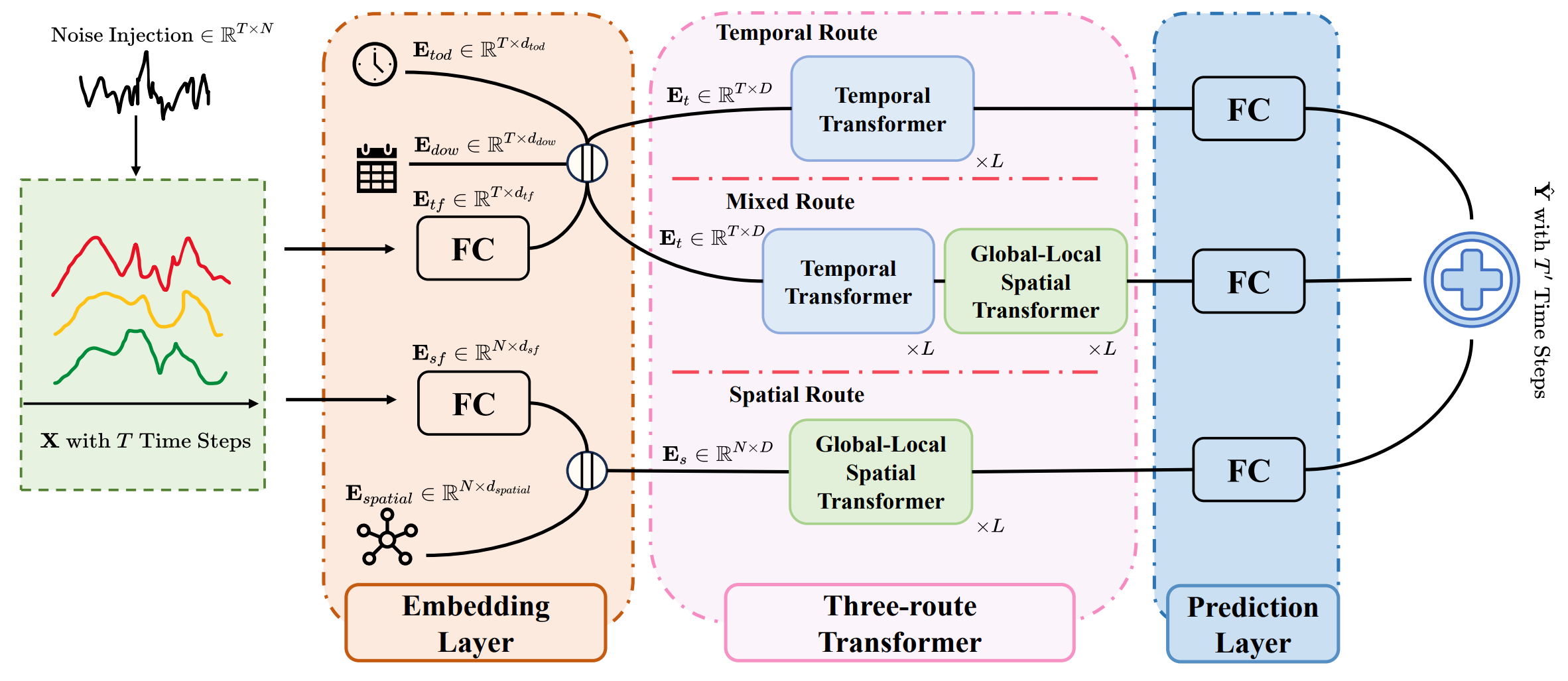
Our project is evolving as a gradual progression from the simple to the complex, from individual elements to a cohesive architecture. Initially, we focused on the conceptual foundation of Extralonger and took the first practical steps toward implementing it using MQL5. At this stage, we implemented spatial and temporal encoding modules, which enabled us to anchor the data to the market structure and lay the groundwork for further integration.

We then moved on to the framework's architectural design. Whereas previously we worked mainly with bricks, we have now started building walls and floor slabs. We examined the implementation of the Global-Local Spatial Transformer module in detail. At this stage, we were able to integrate individual elements into a cohesive computational process. In other words, we have begun to build the very observation framework that will eventually enable us to capture the market in all its dimensions.

These two steps can be compared to setting the stage for a major production. First, we arranged the scenery and determined where the key elements would be placed; then we brought the first actors — the data processing modules — onto the stage. And now we have the opportunity to reveal the entire concept behind the production to the audience. We now move on to the algorithm itself — the heart of Extralonger. It is precisely here — at the intersection of global-local attention, a unified representation, and three parallel routes — that the uniqueness of this approach becomes apparent.

Top-Level Object

At the top of the entire hierarchy of our implementation of the approaches of the Extralonger framework is the CNeuronExtralonger object, which can be viewed as the heart of the architecture, uniting key modules into a single computational cycle. While the classes and blocks discussed earlier were responsible for individual structural elements, here we are dealing with a central node that ties everything together.

class CNeuronExtralonger   :  public CNeuronMHAttentionPooling
  {
protected:
   CLayer               cProjectionT;
   CLayer               cTimeModule;
   CLayer               cSpatialModule;
   CLayer               cMixModule;
   CNeuronBaseOCL       cConcatResults;
   //---
   virtual bool      feedForward(CNeuronBaseOCL *NeuronOCL) override {return false;}
   virtual bool      feedForward(CNeuronBaseOCL *NeuronOCL, CBufferFloat *SecondInput) override;
   virtual bool      updateInputWeights(CNeuronBaseOCL *NeuronOCL) override;
   virtual bool      calcInputGradients(CNeuronBaseOCL *NeuronOCL) override {return false;}
   virtual bool      calcInputGradients(CNeuronBaseOCL *NeuronOCL,
                                        CBufferFloat *SecondInput,
                                        CBufferFloat *SecondGradient,
                                        ENUM_ACTIVATION SecondActivation = None
                                       ) override;

public:
                     CNeuronExtralonger(void) {};
                    ~CNeuronExtralonger(void) {};
   //---
   virtual bool      Init(uint numOutputs, uint myIndex, COpenCLMy *open_cl,
                          uint time_steps_in, uint time_steps_out, uint variables,
                          uint dimension, uint emb_dimension, uint period1,
                          uint frame1, uint period2, uint frame2, uint layers,
                          uint heads, uint dimension_k, uint m_units, float sparse,
                          ENUM_OPTIMIZATION optimization_type, uint batch);
   //---
   virtual int       Type(void)   const   {  return defNeuronExtralonger;   }
   //--- methods for working with files
   virtual bool      Save(int const file_handle) override;
   virtual bool      Load(int const file_handle) override;
   //---
   virtual bool      WeightsUpdate(CNeuronBaseOCL *source, float tau) override;
   virtual void      SetOpenCL(COpenCLMy *obj) override;
   virtual void      SetActivationFunction(ENUM_ACTIVATION value) override { };
  };

Structurally, CNeuronExtralonger inherits from the CNeuronMHAttentionPooling class, which immediately indicates its functional orientation. Data processing remains based on a multi-head attention mechanism with an aggregation mechanism, with additional layers superimposed on top of it to implement Extralonger's unique ideas.

And this brings us to an important difference between our implementation and the original design. In the original version of Extralonger, the emphasis weights for the three data-flow routes (temporal, spatial, and mixed) are hard-coded and remain fixed. This approach is convenient because of its simplicity, but in the context of volatile financial markets, it inevitably leads to a loss of flexibility. In some situations, short-term temporal patterns play a key role; in others, global spatial correlations are crucial; and sometimes, a combination of the two is decisive. Fixed weights cannot dynamically account for this shift in emphasis, which reduces forecast accuracy.

That is precisely why, in our implementation, we went further and introduced an adaptive Attention Pooling mechanism borrowed from the R-MAT framework. The key point is that the weighting coefficients for the routes are not determined in advance but are computed while the model is running. Each new input data signal receives its own attention distribution across the temporal, spatial, and mixed modules. As a result, the system becomes sensitive to the market context. During a phase of calm consolidation, the role of temporal analysis increases; during external shocks, spatial relationships become more important; and during periods of high volatility, the mixed route comes to the fore.

This solution turns CNeuronExtralonger into a much more dynamic tool. Unlike the original static scheme, where the attention distribution is always the same, adaptive Attention Pooling makes the system flexible and self-adjusting. It behaves like an experienced trader who knows how to shift emphasis depending on the situation.

The object contains four key components, which are dynamic arrays. They collect sequences of neural layers from the internal information flows. At first glance, it might seem strange to create four internal modules. After all, the Extralonger architecture mentions only three branches — temporal, spatial, and mixed. It is important to note one particular feature here. The temporal and mixed analysis branches use the same data preparation block. To avoid duplication and improve manageability, we decided to separate the data preparation block into a standalone component — cProjectionT. Essentially, it is a general-purpose gateway that ensures the consistent conversion of input sequences into embeddings suitable for further processing.

We combined the spatial analysis branch with the corresponding data preparation module into a single unit — cSpatialModule. This step is dictated by the specific nature of spatial dependencies. Here, the data preprocessing and the model itself are so closely intertwined that it makes sense to consider them as a single internal structure.

Thus, we end up with four components:

• cProjectionT — the data preparation block for the temporal and mixed branches,
• cTimeModule — a temporal analysis model,
• cSpatialModule — an integrated model for data preparation and spatial analysis,
• cMixModule — a mixed route that integrates temporal and spatial features.

It is precisely this organization that allows us to preserve the logic of the original Extralonger architecture while making the implementation more modular and easier to maintain.

From the overall architectural framework, we gradually move on to its internal details, and it is here that the true complexity of the structure becomes apparent. At the top level, we see only four dynamic arrays — the preparatory temporal-projection block, the temporal module, the spatial module, and the mixed route. But behind this neat facade lies an entire ecosystem of smaller components: convolutional and normalization layers, transposition converters, learnable embeddings, and attention blocks. They do not exist in isolation; each one plays a strictly defined role, and their interaction forms a dynamic flow of information that passes through CNeuronExtralonger.

This entire internal world is created in the Init method. It can be said that this is where the structure and logic of the model's behavior are established. Initialization begins by calling the method of the same name in the parent class, which provides the general framework for multi-head Attention Pooling.

bool CNeuronExtralonger::Init(uint numOutputs, uint myIndex, COpenCLMy *open_cl,
                              uint time_steps_in, uint time_steps_out, uint variables,
                              uint dimension, uint emb_dimension, uint period1,
                              uint frame1, uint period2, uint frame2, uint layers,
                              uint heads, uint dimension_k, uint m_units, float sparse,
                              ENUM_OPTIMIZATION optimization_type, uint batch)
  {
   if(!CNeuronMHAttentionPooling::Init(numOutputs, myIndex, open_cl, variables, time_steps_out,
                                       3, optimization_type, batch))
      return false;

And then the most interesting part begins. Step by step, we assemble a complex organism, where each layer adds its own nuance to the overall picture. But first, a little preparatory work: let's declare a few local variables to temporarily store pointers to objects.

   CNeuronBatchNormOCL           *norm    = NULL;
   CNeuronConvOCL                *conv    = NULL;
   CNeuronTransposeOCL           *transp  = NULL;
   CNeuronLearnabledPE           *lnoise  = NULL;
   CNeuronSpatialEmbedding       *semb    = NULL;
   CNeuronTempEmbedding          *temb    = NULL;
   CNeuronMLMHAttentionOCL       *att     = NULL;
   CNeuronGlobalLocalAttention   *glatt   = NULL;

First on stage is the block for preparing input data for the temporal and mixed analysis branches. It is like a tuner preparing the instruments before a concert. The positional encoding object adds a trainable offset to the input data stream, which the framework's authors call trainable noise. It is important to emphasize here: this is not a random admixture, but a deliberate attempt to build into the model the ability to perceive the market's temporal rhythm. Price and volume data are never clean; they are always swayed by microfluctuations. Embedding trainable noise turns this property into a tool: the model begins to better distinguish patterns from chaos and build its perception of time based on real market rhythms.

//--- Time projection
   cProjectionT.Clear();
   cProjectionT.SetOpenCL(OpenCL);
   int index = 0;
   lnoise = new CNeuronLearnabledPE();
   if(!lnoise ||
      !lnoise.Init(0, index, OpenCL, time_steps_in * variables, optimization, iBatch) ||
      !cProjectionT.Add(lnoise))
     {
      DeleteObj(lnoise);
      return false;
     }

Immediately after it comes a convolutional layer, which plays a special role. It converts each time step into an embedding that contains information about all the analyzed features at that exact moment in time. Essentially, the output forms a compact and informative representation that becomes a kind of snapshot of the market state for each step. Price, volumes, indicators, and other variables are combined into a single vector. In this way, the model can work not with isolated numbers, but with holistic representations that reflect the full spectrum of observations over time.

   index++;
   conv = new CNeuronConvOCL();
   if(!conv ||
      !conv.Init(0, index, OpenCL, variables, variables, dimension, time_steps_in, 1,
                 optimization, iBatch) ||
      !cProjectionT.Add(conv))
     {
      DeleteObj(conv);
      return false;
     }
   conv.SetActivationFunction(None);

The next step is temporal embedding, where the series receive an additional dimension that reflects cycles and periods. The architecture builds in two types of repetition here: short-term and longer-term patterns associated with the market’s daily and weekly rhythms. It is like the way a musician senses the beat and the time signature. Regardless of the melody, there is always a rhythmic foundation without which it is impossible to construct a composition. In financial data, this is reflected in shifts in trading sessions, seasonal fluctuations, or regular patterns of activity among major market participants. Temporal embedding literally stitches this rhythm into the data, making the model sensitive to patterns that repeat from day to day or week to week.

   index++;
   temb = new CNeuronTempEmbedding();
   uint half_emb = (emb_dimension + 1) / 2;
   if(!temb ||
      !temb.Init(0, index, OpenCL, time_steps_in, dimension, half_emb, period1,
                 frame1, dimension - half_emb, period2, frame2, optimization, iBatch) ||
      !cProjectionT.Add(temb))
     {
      DeleteObj(temb);
      return false;
     }

Normalization concludes the preparatory phase. It can be compared to smoothing out a canvas before applying paint. If the surface is uneven, the image will be distorted. Normalization eliminates random distortions, brings the data into a stable distribution, and thereby lays the foundation for further processing by more complex modules.

   index++;
   norm = new CNeuronBatchNormOCL();
   if(!norm ||
      !norm.Init(0, index, OpenCL, temb.Neurons(), iBatch, optimization) ||
      !cProjectionT.Add(norm))
     {
      DeleteObj(norm);
      return false;
     }

When the data leave the preparatory block, they end up in the hands of the temporal analysis module. This is where multi-head attention comes into play, revealing several parallel perspectives at once. It looks for connections between points in time separated by dozens of steps and learns to recognize patterns that are not apparent to a simple, linear view.

//--- Temporal Module
   cTimeModule.Clear();
   cTimeModule.SetOpenCL(OpenCL);
   index++;
   att = new CNeuronMLMHAttentionOCL();
   if(!att ||
      !att.Init(0, index, OpenCL, dimension + emb_dimension, dimension_k, heads,
                time_steps_in, layers, optimization, iBatch) ||
      !cTimeModule.Add(att))
     {
      DeleteObj(att);
      return false;
     }

Next, the block that projects the data onto a specified planning horizon is activated. It can be compared to a bridge connecting historical data with the future. It includes several convolutional layers that transform the embeddings into a multimodal time-series sequence and, at the same time, adjust the sequence length by extending it to the required planning horizon. These layers act as lenses with different depths of field: some emphasize local movements, while others build a broad perspective.

   index++;
   conv = new CNeuronConvOCL();
   if(!conv ||
      !conv.Init(0, index, OpenCL, dimension + emb_dimension, dimension + emb_dimension,
                 variables, time_steps_in, 1, optimization, iBatch) ||
      !cTimeModule.Add(conv))
     {
      DeleteObj(conv);
      return false;
     }
   conv.SetActivationFunction(TANH);
   index++;
   transp = new CNeuronTransposeOCL();
   if(!transp ||
      !transp.Init(0, index, OpenCL, time_steps_in, variables, optimization, iBatch) ||
      !cTimeModule.Add(transp))
     {
      DeleteObj(transp);
      return false;
     }
   index++;
   conv = new CNeuronConvOCL();
   if(!conv ||
      !conv.Init(0, index, OpenCL, time_steps_in, time_steps_in, time_steps_out, variables,
                 1, optimization, iBatch) ||
      !cTimeModule.Add(conv))
     {
      DeleteObj(conv);
      return false;
     }
   conv.SetActivationFunction(SoftPlus);
   index++;
   conv = new CNeuronConvOCL();
   if(!conv ||
      !conv.Init(0, index, OpenCL, time_steps_out, time_steps_out, time_steps_out, variables,
                 1, optimization, iBatch) ||
      !cTimeModule.Add(conv))
     {
      DeleteObj(conv);
      return false;
     }
   conv.SetActivationFunction(None);
   index++;
   norm = new CNeuronBatchNormOCL();
   if(!norm ||
      !norm.Init(0, index, OpenCL, conv.Neurons(), iBatch, optimization) ||
      !cTimeModule.Add(norm))
     {
      DeleteObj(norm);
      return false;
     }
   index++;
   transp = new CNeuronTransposeOCL();
   if(!transp ||
      !transp.Init(0, index, OpenCL, variables, time_steps_out, optimization, iBatch) ||
      !cTimeModule.Add(transp))
     {
      DeleteObj(transp);
      return false;
     }

The result is no longer just a set of embeddings, but a forecast trajectory adapted to the planning horizon.

At the same time, the mixed module begins to operate, and it is here that the data undergo a particularly eventful journey. Its role is unique: to combine temporal and spatial features, transforming them into a single stream of information. The first to come into play is a classic multi-head attention block, which analyzes the temporal sequence in its pure form. It looks for patterns, correspondences, and recurring motifs hidden in the structure of the sequence, thereby creating a solid framework for further analysis.

//--- Mixed Module
   cMixModule.Clear();
   cMixModule.SetOpenCL(OpenCL);
   uint att_layers = (layers + 1) / 2;
   index++;
   att = new CNeuronMLMHAttentionOCL();
   if(!att ||
      !att.Init(0, index, OpenCL, dimension + emb_dimension, dimension_k, heads,
                time_steps_in, att_layers, optimization, iBatch) ||
      !cMixModule.Add(att))
     {
      DeleteObj(att);
      return false;
     }

The data then undergoes transposition, a sort of shift in perspective. While we initially viewed the time series in terms of time steps, the focus now shifts to features, and it is within this new coordinate system that the global-local attention module comes into play. Here, two opposing perspectives are balanced: a global view that encompasses the entire market, and a local focus that makes it possible to discern subtle connections between individual instruments or short-lived spikes. This combination is particularly important in a financial context: the market may move within the bounds of a major trend for weeks, but individual assets can suddenly change direction due to news or local events.

   index++;
   transp = new CNeuronTransposeOCL();
   if(!transp ||
      !transp.Init(0, index, OpenCL, time_steps_in, dimension + emb_dimension, optimization, iBatch) ||
      !cMixModule.Add(transp))
     {
      DeleteObj(transp);
      return false;
     }
   for(uint i = (att_layers == layers ? 0 : att_layers - 1); i < layers; i++)
     {
      index++;
      glatt = new CNeuronGlobalLocalAttention();
      if(!glatt ||
         !glatt.Init(0, index, OpenCL, dimension + emb_dimension, time_steps_in, dimension_k, heads,
                     m_units, sparse, optimization, iBatch) ||
         !cMixModule.Add(glatt))
        {
         DeleteObj(glatt);
         return false;
        }
     }

The final step is the forecasting block, which is responsible for converting all the accumulated information into a format suitable for planning over a specified planning horizon. Several convolutional layers in this block transform the embeddings into a sequence of forecast values that matches the length of the required window. It is here that abstract representations are transformed into a concrete result — a forecast that reflects both the global context and local characteristics.

   index++;
   conv = new CNeuronConvOCL();
   if(!conv ||
      !conv.Init(0, index, OpenCL, time_steps_in, time_steps_in, time_steps_out,
                             dimension + emb_dimension, 1, optimization, iBatch) ||
      !cMixModule.Add(conv))
     {
      DeleteObj(conv);
      return false;
     }
   conv.SetActivationFunction(SoftPlus);
   index++;
   conv = new CNeuronConvOCL();
   if(!conv ||
      !conv.Init(0, index, OpenCL, time_steps_out, time_steps_out, time_steps_out,
                 dimension + emb_dimension, 1, optimization, iBatch) ||
      !cMixModule.Add(conv))
     {
      DeleteObj(conv);
      return false;
     }
   conv.SetActivationFunction(TANH);
   index++;
   transp = new CNeuronTransposeOCL();
   if(!transp ||
      !transp.Init(0, index, OpenCL, dimension + emb_dimension, time_steps_out,
                                                          optimization, iBatch) ||
      !cMixModule.Add(transp))
     {
      DeleteObj(transp);
      return false;
     }
   index++;
   conv = new CNeuronConvOCL();
   if(!conv ||
      !conv.Init(0, index, OpenCL, dimension + emb_dimension, dimension + emb_dimension,
                                     variables, time_steps_out, 1, optimization, iBatch) ||
      !cMixModule.Add(conv))
     {
      DeleteObj(conv);
      return false;
     }
   conv.SetActivationFunction(None);
   index++;
   norm = new CNeuronBatchNormOCL();
   if(!norm ||
      !norm.Init(0, index, OpenCL, conv.Neurons(), iBatch, optimization) ||
      !cMixModule.Add(norm))
     {
      DeleteObj(norm);
      return false;
     }

As a result, the mixed module functions as a synthesis laboratory: first, temporal patterns are captured; then they are superimposed on spatial relationships; and finally, the resulting signal passes through a forecasting block and becomes a full-fledged output in which several levels of analysis are interwoven.

The final stage of the data's internal journey is the spatial module. It is responsible for ensuring that the market is no longer viewed as a collection of independent time series. First, spatial embeddings are formed here; they capture the long-term relationships between instruments, sectors, and indices.

//--- Spatial Module
   cSpatialModule.Clear();
   cSpatialModule.SetOpenCL(OpenCL);
   index++;
   transp = new CNeuronTransposeOCL();
   if(!transp ||
      !transp.Init(0, index, OpenCL, time_steps_in, variables, optimization, iBatch) ||
      !cSpatialModule.Add(transp))
     {
      DeleteObj(transp);
      return false;
     }
   index++;
   conv = new CNeuronConvOCL();
   if(!conv ||
      !conv.Init(0, index, OpenCL, time_steps_in, time_steps_in, dimension, variables,
                 1, optimization, iBatch) ||
      !cSpatialModule.Add(conv))
     {
      DeleteObj(conv);
      return false;
     }
   conv.SetActivationFunction(None);
   index++;
   semb = new CNeuronSpatialEmbedding();
   if(!semb ||
      !semb.Init(0, index, OpenCL, variables, dimension, emb_dimension, optimization, iBatch) ||
      !cSpatialModule.Add(semb))
     {
      DeleteObj(semb);
      return false;
     }

Based on these, the global-local attention blocks sequentially build a broad picture of correlations and detailed relationships between specific assets. It can be said that this module transforms the financial market into a living network, where each link is connected to the others, and it is this network that becomes the object of analysis.

   index++;
   norm = new CNeuronBatchNormOCL();
   if(!norm ||
      !norm.Init(0, index, OpenCL, semb.Neurons(), iBatch, optimization) ||
      !cSpatialModule.Add(norm))
     {
      DeleteObj(norm);
      return false;
     }
   for(uint i = 0; i < layers; i++)
     {
      index++;
      glatt = new CNeuronGlobalLocalAttention();
      if(!glatt ||
         !glatt.Init(0, index, OpenCL, dimension + emb_dimension, variables, dimension_k,
                     heads, m_units, sparse, optimization, iBatch) ||
         !cSpatialModule.Add(glatt))
        {
         DeleteObj(glatt);
         return false;
        }
     }

And, as with the two pathways presented above, the results of the analysis are sent to the forecasting block, which carefully packages all the information into a format suitable for planning over a specified period.

   index++;
   conv = new CNeuronConvOCL();
   if(!conv ||
      !conv.Init(0, index, OpenCL, dimension + emb_dimension, dimension + emb_dimension,
                 time_steps_out, variables, 1, optimization, iBatch) ||
      !cSpatialModule.Add(conv))
     {
      DeleteObj(conv);
      return false;
     }
   conv.SetActivationFunction(SoftPlus);
   index++;
   conv = new CNeuronConvOCL();
   if(!conv ||
      !conv.Init(0, index, OpenCL, time_steps_out, time_steps_out, time_steps_out,
                 variables, 1, optimization, iBatch) ||
      !cSpatialModule.Add(conv))
     {
      DeleteObj(conv);
      return false;
     }
   conv.SetActivationFunction(None);
   index++;
   norm = new CNeuronBatchNormOCL();
   if(!norm ||
      !norm.Init(0, index, OpenCL, conv.Neurons(), iBatch, optimization) ||
      !cMixModule.Add(norm))
     {
      DeleteObj(norm);
      return false;
     }
   index++;
   transp = new CNeuronTransposeOCL();
   if(!transp ||
      !transp.Init(0, index, OpenCL, variables, time_steps_out, optimization, iBatch) ||
      !cMixModule.Add(transp))
     {
      DeleteObj(transp);
      return false;
     }

All three routes (temporal, mixed, and spatial) converge at the concatenation point. This is where their results are combined, and it is at this stage that our key mechanism — adaptive Attention Pooling — is activated. Unlike the original version with fixed weights, we allow the routes to determine among themselves whose role is more important at any given moment. As a result, the final signal is not a static construct, but a flexible tool that breathes in rhythm with the market.

   index++;
   if(!cConcatResults.Init(0, index, OpenCL, 3 * variables * time_steps_out, optimization, iBatch))
      return false;
   cConcatResults.SetActivationFunction(None);
//---
   return true;
  }

Thus, the Init method transforms a dry sequence of calls into a dynamic architecture, where each component plays a meaningful role and their interaction gives rise to a unique analysis tool. This is where an organism called CNeuronExtralonger comes into being, and every part of it works toward the overall result.

After initializing the object, we move on to building the forward-pass algorithm, which is implemented in the feedForward method. The method signature speaks volumes on its own. As parameters, it receives a pointer to the source data object NeuronOCL and an additional buffer, SecondInput, containing the timestamps of the sequence being analyzed.

bool CNeuronExtralonger::feedForward(CNeuronBaseOCL *NeuronOCL, CBufferFloat *SecondInput)
  {
   CNeuronBaseOCL *prev = NeuronOCL;
   CNeuronBaseOCL *current = NULL;

The first internal operation is the declaration of two local variables. One of them is assigned a pointer to the source data object. This is a standard pass-through technique: prev serves as the last available result, which is passed to the next layer. And current serves as a temporary variable into which a pointer to the layer being processed is stored at each iteration. This approach makes it possible to build a chain of layers linearly, avoiding unnecessary copying and maintaining control over the sequence of computations.

Next, a loop is started over the source data preparation container cProjectionT. For each projection, we take a pointer to the current object and immediately check its pointer validity. Next, we call the object's forward-pass method. If an error occurs at any stage, the method immediately terminates and returns false. This is a fail-fast pattern: it is better to stop at the first problem than to continue processing corrupted data.

//--- Time projection
   for(int i = 0; i < cProjectionT.Total(); i++)
     {
      current = cProjectionT[i];
      if(!current ||
         !current.FeedForward(prev, SecondInput))
         return false;
      prev = current;
     }

It is important to note that in this block, the FeedForward method of the internal objects takes two arguments: the previous result and the SecondInput timestamps. After all, generating temporal embeddings requires additional context.

If everything went well, the prev variable is updated to point to current, so that the next iteration operates on the output of the layer that was just processed.

When the projections are complete, control is transferred to the temporal module. The loop over the cTimeModule container looks almost the same, but here the FeedForward method of the internal objects is called with only one argument. This indicates that the temporal module processes the resulting sequence without an additional buffer.

//--- Temporal Module
   for(int i = 0; i < cTimeModule.Total(); i++)
     {
      current = cTimeModule[i];
      if(!current ||
         !current.FeedForward(prev))
         return false;
      prev = current;
     }

If any layer of the temporal module is missing, or if its FeedForward signals an error, we again terminate processing and return false.

Then the focus shifts to the mixed module. However, it should be remembered that this module also works with the results of data preprocessing; therefore, before starting the loop, we set the prev variable to a pointer to the last layer of the cProjectionT container. The temporal and mixed branches follow parallel paths, processing the same input features in different ways.

//--- Mixed Module
   prev = cProjectionT[-1];
   for(int i = 0; i < cMixModule.Total(); i++)
     {
      current = cMixModule[i];
      if(!current ||
         !current.FeedForward(prev))
         return false;
      prev = current;
     }

Next, for each element of cMixModule, the same pointer validity check is performed and the forward-pass method is called, followed by updating the pointer in prev. Any error will again cause the function to terminate immediately and return false.

The spatial module is organized separately and receives NeuronOCL as its input data. This means that the Spatial branch analyzes the input signal in parallel with the other branches, without inheriting the intermediate transformations. The cSpatialModule layers are then run sequentially, using the usual fail-fast logic and updating prev.

//--- Spatial Module
   prev = NeuronOCL;
   for(int i = 0; i < cSpatialModule.Total(); i++)
     {
      current = cSpatialModule[i];
      if(!current ||
         !current.FeedForward(prev))
         return false;
      prev = current;
     }

As a result, we end up with three complete branches: temporal, mixed, and spatial. The next step is concatenation. We combine the outputs of the three branches into a single buffer, forming a window and setting the final dimensionality. If the concatenation fails, the method returns false.

//--- Concatenate
   if(!Concat(cTimeModule[-1].getOutput(), cMixModule[-1].getOutput(), cSpatialModule[-1].getOutput(),
              cConcatResults.getOutput(), iWindow, iWindow, iWindow, iUnits))
      return false;
//---
   return CNeuronMHAttentionPooling::feedForward(cConcatResults.AsObject());
  }

After successful concatenation, the aggregated result must be passed to the Attention Pooling module.

Architecturally, it is clear that the system is built as a set of parallel pathways, each of which examines the input data with its own purpose: the projections prepare temporal representations, the temporal module analyzes the sequence, the mixed module combines the projections, and the Spatial module focuses on spatial features. This scheme is similar to an orchestra: each instrument has its own part, and the conductor — Attention Pooling — brings it all together.

The error-gradient propagation method largely mirrors the structure of the forward pass, with the difference that the data flows in the opposite direction and the error streams must be carefully summed.

bool CNeuronExtralonger::calcInputGradients(CNeuronBaseOCL *NeuronOCL,
                                            CBufferFloat *SecondInput,
                                            CBufferFloat *SecondGradient,
                                            ENUM_ACTIVATION SecondActivation = None)
  {
   if(!NeuronOCL)
      return false;
//---
   if(!CNeuronMHAttentionPooling::calcInputGradients(cConcatResults.AsObject()))
      return false;

First, we check the validity of the pointer to the source data object. If it is empty, the method immediately returns false. Next, the method of the same name in the parent class is called. This step allows the error gradient received from the subsequent neural layer to be propagated down to the concatenated buffer. The obtained values are then distributed back across the three branches — temporal, mixed, and spatial. It is important to note that the error collected in the shared buffer is divided strictly in accordance with the model's architecture. Each branch has been assigned the correct gradient. If any of the operations fails, the process is interrupted.

//--- DeConcatenate
   if(!cTimeModule[-1] || !cMixModule[-1] || !cSpatialModule[-1] ||
      !DeConcat(cTimeModule[-1].getGradient(), cMixModule[-1].getGradient(),
                cSpatialModule[-1].getGradient(), cConcatResults.getOutput(),
                iWindow, iWindow, iWindow, iUnits))
      return false;

Next, the gradients begin to propagate through the modules in reverse order. First, the spatial branch. The loop runs from the end to the beginning; each current element retrieves a reference to the next layer and calls the error-gradient propagation method of the internal object. The error is carefully pushed back, layer by layer.

   CNeuronBaseOCL *next = NULL;
   CNeuronBaseOCL *current = NULL;
//--- Spatial Module
   for(int i = cSpatialModule.Total() - 1; i >= 0; i--)
     {
      current = (i > 0 ? cSpatialModule[i - 1] : NeuronOCL);
      next = cSpatialModule[i];
      if(!current ||
         !current.CalcHiddenGradients(next))
         return false;
     }

The same logic applies to the mixed module, except that here the last element of the temporal projections is used as the reference point. This reflects the model's parallel structure: different branches return errors through their own channels, but always synchronously.

//--- Mixed Module
   for(int i = cMixModule.Total() - 1; i >= 0; i--)
     {
      current = (i > 0 ? cMixModule[i - 1] : cProjectionT[-1]);
      next = cMixModule[i];
      if(!current ||
         !current.CalcHiddenGradients(next))
         return false;
     }

The temporal module is of particular interest. It is worth noting here that it passes the error gradient to the last layer of the data preprocessing module. And that is exactly where we just passed the values from the mixed module. Therefore, before performing the backward pass of the temporal analysis module, we store a pointer to the current error-gradient buffer containing the saved values in the local variable temp. We then pass a pointer to a free buffer to the object.

//--- Temporal Module
   CBufferFloat *temp = current.getGradient();
   if(!current.SetGradient(current.getPrevOutput(), false))
      return false;
   for(int i = cTimeModule.Total() - 1; i >= 0; i--)
     {
      current = (i > 0 ? cTimeModule[i - 1] : cProjectionT[-1]);
      next = cTimeModule[i];
      if(!current ||
         !current.CalcHiddenGradients(next))
         return false;
     }
   if(!SumAndNormilize(temp, current.getGradient(), temp, 1, false, 0, 0, 0, 1) ||
      !current.SetGradient(temp, false))
      return false;

Next, in the loop, again from end to beginning, the gradients are propagated down through the module. After completing the backward pass along the temporal branch, we sum the values obtained from the two data streams and restore the data-buffer pointers to their original state.

The final step is to process the temporal projections. Here, the gradient descends to the level of the source data object. However, I would like to remind you that we have already sent the error gradients from the spatial branch there. Therefore, we repeat the trick of swapping the data buffer and then perform the error-gradient propagation operations.

//--- Time projection
   temp = NeuronOCL.getGradient();
   if(!NeuronOCL.SetGradient(NeuronOCL.getPrevOutput(), false))
      return false;
   for(int i = cProjectionT.Total() - 1; i >= 0; i--)
     {
      current = (i > 0 ? cProjectionT[i - 1] : NeuronOCL);
      next = cProjectionT[i];
      if(!current ||
         !current.CalcHiddenGradients(next, SecondInput, SecondGradient, SecondActivation))
         return false;
     }
   if(!SumAndNormilize(temp, NeuronOCL.getGradient(), temp, 1, false, 0, 0, 0, 1) ||
      !NeuronOCL.SetGradient(temp, false))
      return false;
//---
   return true;
  }

Thus, the method carefully distributes the gradients across three parallel branches — Spatial, Mix, and Temporal. In each branch, the backward pass proceeds layer by layer in reverse order, and the errors are summed at the branch junctions. This reflects the same architectural concept as in the forward pass: data flows through parallel channels but is ultimately combined into a single result.

The complete class code, including all methods, is provided in the attachment, allowing you to examine the overall structure and the inner workings of the implementation.

Model Architecture

Once we have finished building all the necessary objects for implementing the Extralonger framework, the next logical step is to describe the architecture of the model itself. It is important to emphasize here that we do not limit ourselves to forecasting time series, as is done in the author's implementation. Our goal is broader and more practical — we are developing a full-fledged trading robot capable of making decisions independently and executing trades in the market.

In this formulation, the task of forecasting price series ceases to be the ultimate goal and serves only as part of the system — specifically, as an Encoder of the environment state. A kind of sensor that converts market data into a format that the algorithm can understand. While retaining the Actor–Critic concept, we develop three functional models: Encoder, Actor, and Critic.

The CreateDescriptions method is used to describe their architecture. In it, arrays containing layer descriptions are carefully created and initialized for each of the three parts of the model.

bool CreateDescriptions(CArrayObj *&encoder,
                        CArrayObj *&actor,
                        CArrayObj *&critic
                       )
  {
//---
   CLayerDescription *descr;
//---
   if(!encoder)
     {
      encoder = new CArrayObj();
      if(!encoder)
         return false;
     }
   if(!actor)
     {
      actor = new CArrayObj();
      if(!actor)
         return false;
     }
   if(!critic)
     {
      critic = new CArrayObj();
      if(!critic)
         return false;
     }

The code begins by checking the received array pointers. If one of them does not yet exist, a new one is created. This step ensures reliability — we guarantee that further filling in the descriptions will not cause failures due to a missing structure.

Next, the arrays are cleared, and the layers of the Encoder are constructed step by step. The source data layer is added first.

//--- Encoder
   encoder.Clear();
//--- Input layer
   if(!(descr = new CLayerDescription()))
      return false;
   descr.type = defNeuronBaseOCL;
   uint prev_count = descr.count = (HistoryBars * BarDescr);
   descr.activation = None;
   descr.optimization = ADAM;
   if(!encoder.Add(descr))
     {
      delete descr;
      return false;
     }

The next step is a normalization layer with added noise, which helps improve training stability through stochastic distortions.

//--- Layer 1
   if(!(descr = new CLayerDescription()))
      return false;
   descr.type = defNeuronBatchNormWithNoise;
   descr.count = prev_count;
   descr.batch = BatchSize;
   descr.activation = None;
   descr.optimization = ADAM;
   if(!encoder.Add(descr))
     {
      delete descr;
      return false;
     }

Next, a layer is created to add first-order difference features. Its purpose is to generate time slices by linking the values of the bars together. As a result, this layer produces twice as many features, since the values themselves and their differences are combined.

//--- Layer 2
   if(!(descr = new CLayerDescription()))
      return false;
   descr.type = defNeuronConcatDiff;
   prev_count = descr.count = HistoryBars;
   descr.layers = BarDescr;
   descr.step = 1;
   descr.batch = BatchSize;
   descr.optimization = ADAM;
   descr.activation = None;
   if(!encoder.Add(descr))
     {
      delete descr;
      return false;
     }
   uint prev_out = descr.layers*2 ;

The next layer, defNeuronExtralonger, is of particular interest. It defines the architecture of the top-level CNeuronExtralonger object we have created. Essentially, this is the entire Extralonger framework. In it, we specify all the necessary parameters: time windows, the forecast horizon, short and long periods, and the dimensionality of the hidden features. This block transforms the Encoder into an intelligent filter that connects historical data and the future within a unified representation.

//--- Layer 3
   if(!(descr = new CLayerDescription()))
      return false;
   descr.type = defNeuronExtralonger;
     {
      uint temp[] = {HistoryBars,   // History time steps
                     NForecast,     // Forecast time steps
                     ShortPeriod,   // Period 2
                     LongPeriod,    // Period 2
                     BarDescr/2     // M units
                    };
      if(ArrayCopy(descr.units, temp) < (int)temp.Size())
         return false;
     }
   prev_count = descr.units[1];
   descr.window = prev_out;            // Variables
   descr.window_out = EmbeddingSize;   // Inside Dimension
     {
      uint temp[] = {EmbeddingSize,             // Embedding Dimension
                     PeriodSeconds(PERIOD_H1),  // Frame 1
                     PeriodSeconds(PERIOD_D1),  // Frame 2
                     2*EmbeddingSize/NHeads
                    };
      if(ArrayCopy(descr.windows, temp) < (int)temp.Size())
         return false;
     }
   descr.layers=2;
   descr.step=NHeads;
   descr.probability=0.3f;
   descr.optimization=ADAM;
   descr.batch=BatchSize;
   descr.activation = None;
   if(!encoder. Add(descry))
     {
      delete descry;
      return false;
     }
   uint window=descr.window;
   uint count=prev_count; 

At the output of the Extralonger module, we obtain an already formed block of forecast values, ready for further use. But it is important to remember that even before feeding the data into this module, we had enriched it with first-difference features. This technique made the series more informative, but at the same time increased the dimensionality of the data.

It would seem that the simplest way to solve this problem is to simply discard the excess features. However, this approach would result in the loss of the information that was the very reason the first difference was introduced in the first place. Instead of a simplified solution, we use a convolutional layer, which not only reduces dimensionality but also selects the most significant local patterns. As a result, the module output undergoes fine filtering: the data become more compact while retaining the full range of essential characteristics needed for making trading decisions.

//--- layer 4
   if(!(descr = new CLayerDescription()))
      return false;
   descr.type = defNeuronConvOCL;
   descr.count = prev_count;
   descr.window = prev_out;
   descr.step = prev_out;
   prev_out = descr.window_out = BarDescr;
   descr.activation = TANH;
   descr.optimization = ADAM;
   if(!encoder.Add(descr))
     {
      delete descr;
      return false;
     }

The final component of the Environmental State Encoder is the reverse denormalization layer (defNeuronRevInDenormOCL). This layer returns the values to the scale of the data being analyzed, eliminating the offset that arose during encoding and normalization. Thus, the result becomes comparable to actual market values.

//--- layer 5
   if(!(descr = new CLayerDescription()))
      return false;
   descr.type = defNeuronRevInDenormOCL;
   descr.count = prev_count * prev_out;
   descr.layers = 1;
   if(!encoder.Add(descr))
     {
      delete descr;
      return false;
     }

The architecture of the Actor and Critic models is taken entirely from our previous works and has not undergone any changes. That is precisely why we will not go into detail about it in this article. To complete the picture, readers can find a full description of the architecture of all trainable models in the appendix, where they can follow every implementation detail and verify the integrity of the solution that has been built.

Testing

Model training is comprehensive preparation for trading. Before releasing it into the live market, we thoroughly backtested the strategy on historical data. The first stage — offline training — was conducted on a sample of the EURUSD currency pair on the H1 timeframe for the period from January 2024 to June 2025. This period proved rich and varied: calm phases of sideways markets alternated with sharp trending moves, while high volatility flared up around news releases. This combination of conditions enabled the model to learn to distinguish a wide range of market scenarios and generate robust trading decisions without losing its bearings in complex situations.

Once the first phase of preparation was complete, we moved on to the second — online fine-tuning in the MetaTrader 5 Strategy Tester. Here, data arrived in real time, one candlestick at a time, and the model learned the dynamics of operating on a live data stream. It learned to maintain stability amid market noise, cope with low liquidity, and stay on track during sudden price spikes. This stage served as a kind of strategy refinement. It did not change the framework built on historical data, but it helped adapt it to real-world conditions and reduced the risk of overfitting.

The final test was conducted using data from July 2025 — this data had not been used previously and was completely new to the model. All parameters obtained in the previous stages were loaded without any changes. This clean out-of-sample test made it possible to objectively assess the model's ability to generalize, without any fine-tuning or adjustments.

The test results are presented below.

The test results make it possible to evaluate the model under real-world market conditions without any adjustments. Let's start with the key figures. With an initial deposit of USD 100, the final net result was USD 3.02, meaning the balance grew by three percent over the one-month test period. Total profit reached USD 27.26, and total losses amounted to USD 24.24. Profit Factor was 1.12. This suggests that profitable trades slightly outweigh losing trades.

However, there is also a weakness: the recovery factor is only 0.22. This means that after a series of losses, the model recovers its capital slowly. The maximum balance drawdown was 12.75% — a fairly significant figure, but still not critical for fully automated trading. The average expected value per trade turned out to be modest — USD 0.06 — but the Sharpe Ratio (3.04) indicates a good return-to-risk ratio when volatility is taken into account.

The trade statistics are also interesting. There were 50 trades in total, including 28 short trades (with a success rate of 53.57%) and 22 long trades (successful only 36.36% of the time). Overall, the percentage of profitable trades was 46%. The largest profit on a single trade was USD 6.70, and the largest loss was USD 4.73. The streaks were revealing as well: the model managed to win up to five trades in a row, while losing no more than three.

The capital curve confirms the picture painted by the numbers. The first few days of July were marked by fluctuations and a series of drawdowns, after which the balance began to rise gradually. In the middle of the month, several successful sequences of trades appeared, allowing capital to move into positive territory. Toward the end of July, the situation stabilized and the results held steady, with no new sharp declines.

Thus, the test showed that the model is capable of generating moderate returns while maintaining a balance between risk and return. However, the testing period is quite short, and further optimization will be required for live deployment. First and foremost, this means reducing drawdown and increasing the percentage of profitable trades. But most importantly, the system passed a clean out-of-sample test on new data and demonstrated its ability to generalize, which is a key criterion for the quality of an algorithmic model.

And let's not forget that training transformers is a rather complex process that requires large training datasets.

Conclusion

In the course of our work, we have found that the approaches proposed by the Extralonger framework are capable of seamlessly integrating spatial and temporal factors, thereby forming a solid foundation for analyzing market dynamics.

Testing has confirmed the practical effectiveness of the algorithms, and the flexibility of the architecture allows the system to be adapted to various forecast horizons and classes of financial instruments. Implementation in MQL5 has shown that classical approaches, when combined with modern neural network methods, yield results comparable to those of more complex systems while remaining highly transparent and manageable.

Links

• Extralonger: Toward a Unified Perspective of Spatial-Temporal Factors for Extra-Long-Term Traffic Forecasting
• Other articles in this series

Files used in the article

#	Name	Type	Description
1	Study.mq5	Expert Advisor	Expert Advisor for offline model training
2	StudyOnline.mq5	Expert Advisor	Expert Advisor for online model training
3	Test.mq5	Expert Advisor	Expert Advisor for model testing
4	Trajectory.mqh	Class library	Structure for describing the system state and model architecture
5	NeuroNet.mqh	Class library	Class library for creating a neural network
6	NeuroNet.cl	Library	Code library for an OpenCL program