

Neural Networks in Trading: Robust Trading Signals in Any Market Regime (ST-Expert)
 184
184
 0
0

Introduction
Today's financial markets are a dynamic ecosystem in which millions of transactions, regulatory decisions, corporate reports, and macroeconomic signals come together to form a complex pattern. For a trader or analyst, the key task is to identify regularities in this pattern and use them to build a forecast. But this is precisely where the main contradiction arises: the market is changing faster than traditional models can adapt. What worked yesterday may turn out to be not only useless but also dangerous tomorrow.
We are accustomed to thinking in terms of correlations. There is a stable relationship between the price of oil and the Canadian dollar exchange rate, between the Fed's interest rates and the technology sector, and between demand for gold and movements in the dollar. But as soon as external conditions change, these dependencies collapse. During the COVID-19 market crash of 2020, the usual correlations between stocks, bonds, and commodities ceased to reflect reality in a matter of weeks. Even milder regime shifts, such as cycles of rate hikes and cuts by the Federal Reserve, can drastically alter correlations and undermine models that once seemed reliable.
The crux of the problem is that modern algorithms are trained on relatively short and homogeneous data intervals. Under these laboratory conditions, they deliver impressive results by detecting subtle correlations between assets. But as soon as the market moves beyond its usual distribution, the accuracy of forecasts drops sharply. Essentially, the models work perfectly well during calm periods, but they are unable to handle market phase transitions.
This situation is in many ways reminiscent of urban transportation networks — the example used by the authors of the paper "Robust Traffic Forecasting against Spatial Shift over Years" to propose a new framework, ST-Expert. As long as the city remains unchanged, traffic forecasts work perfectly. But as soon as a new interchange is built or a large shopping center opens, the old routes become obsolete. In the financial environment, these drivers are regulatory decisions, sanctions, geopolitical conflicts, or the emergence of new technologies. The landscape of relationships is changing, and old models are proving ineffective.
To tackle this challenge, the authors of ST-Expert propose an original solution based on Mixture of Experts. Its key idea is that the model learns not from a single rigid structure of dependencies, but from a set of graph generators known as graphons. Each of them reflects a specific type of market behavior. One identifies patterns under a sustained trend, another describes a phase of high volatility, and a third detects local correlations within industries. When the market changes, the system does not break down; instead, it adaptively combines previously learned scenarios, creating new connections between instruments and maintaining forecast accuracy.
This is precisely where the first — and perhaps the main — advantage of this approach becomes evident: its ability to adapt to changing market conditions. If standard models become trapped in a specific historical period, the new framework views the market as a mosaic in which each regime is merely a temporary fragment of the whole. As a result, the algorithm can assemble a new combination from elements it has already learned and deliver an accurate forecast where other systems lose robustness. For a trader, this means fewer false signals during periods of market turbulence and greater reliability when developing long-term strategies.
But adaptability is just one aspect. Another key advantage is the architecture's versatility. The layer of expert graphons can be easily integrated into existing solutions. It can be added both to graph neural networks that analyze network relationships among assets and to transformers that work with time series of price quotes. This makes the approach particularly valuable for practitioners. It does not require a radical overhaul of the infrastructure and can enhance systems that are already well-established.
Another advantage lies in its robustness to so-called regime shifts. The history of financial markets clearly shows that constancy is rare, while change is the rule. Every decade brings a new crisis, and each era within a crisis is accompanied by a cascade of unpredictable shocks. The attempt to find timeless invariants turns out to be an illusion. The new framework openly acknowledges the ever-changing nature of markets and derives its strength precisely from its ability to switch between scenarios. This is particularly important for stress testing and long-term forecasting, where the cost of error is extremely high.
At the same time, the approach remains compact and efficient. In financial applications, time is critical. Trade decisions must be made in milliseconds. Therefore, no matter how accurate models may be, they cannot afford to be excessively computationally heavy. The proposed framework takes this factor into account. It adds flexibility and robustness without a sharp increase in computational costs. As a result, it can be used in real-time systems — from algorithmic trading to risk management.
Finally, it is worth noting its flexibility in terms of extensibility. Expert graphons are not limited to any single market or asset class. They can be used in equities, bonds, currencies, and cryptocurrency markets. Moreover, they can integrate different types of data — from market quotes and news feeds to macroeconomic indicators. This paves the way for building truly comprehensive models that take into account the multilayered nature of financial systems.
This is a fundamentally new perspective on the very nature of modeling under uncertainty. While traditional models persistently seek certain timeless patterns, ST-Expert teaches the system to adapt to a changing world. It transforms forecasting into a dynamic process that can account for unexpected changes and adapt in real time.
ST-Expert Algorithm
Building a reliable predictive model for financial markets requires the ability to distinguish between and account for various market regimes. In reality, the structure of correlations between assets is far from static. What seemed like a robust rule yesterday may turn out to be a mere coincidence tomorrow. During periods of growth in the technology sector, the links between IT company stocks and interest rates may be minimal, but at the first signs of overheating they come to the fore. In commodity markets, the correlation between oil prices and the currencies of exporting countries is particularly pronounced during crisis periods, but may then virtually disappear. It is clear that a model that attempts to reduce all this diversity to a single fixed matrix of relationships is bound to lose accuracy.
That is precisely why the authors propose an approach based on identifying characteristic time segments within which the market behaves in a relatively uniform manner. The idea is simple. If we treat all the historical data as a single dataset, important regimes will be washed out, and no expert will be able to learn them correctly. But if we divide the historical data into periods, each of which has its own robust correlation structure, then a specialized expert can be built for each such period. Subsequently, the model will combine these experts, creating a flexible representation of the market environment.
Formally, this leads to the Maximum Spatiotemporal Graph Division (MSGD) problem. The entire time series (denoted as T) is divided into K non-overlapping intervals. Each interval Tk includes the pairs (Xt, Yt) for t ∈ [tk, tk+1). It is important to note that, within such an interval, market relationships are described by the same structure Rk, whereas these structures differ across different intervals.

Essentially, this means that morning stock market sessions can be similar to one another, even if they take place on different days. Retail investor activity creates one type of correlation, while the evening hours, when institutional participants enter the market, form a completely different pattern of relationships. The idea behind MSGD is to partition the data precisely so that the difference between the identified intervals is maximized.
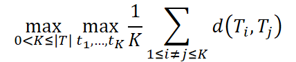
Subject to the following conditions

Here, as a measure of dissimilarity d(•,•), the authors of the framework propose using Kendall’s tau coefficient τ, which reflects the extent to which correlation structures differ across periods. The constraints α1 and α2 specify the minimum and maximum permissible interval lengths, and T is the total duration of the series.
Thus, the task boils down to splitting the historical data into parts that differ most strongly from one another in terms of their types of dependencies. In other words, we are looking for pure market regimes: an uptrend phase, a range-bound phase, and a high-volatility phase. This approach is similar to creating thematic indices. Each index groups together securities of a single type and tracks their performance without mixing it with that of other market segments.
Solving this problem is, of course, not easy. It cannot be expressed analytically, so the framework's authors resort to dynamic programming. This makes it possible to efficiently determine both the number of intervals K and their boundaries, even when dealing with large amounts of data.
Once the periods have been defined, the question arises: how exactly should we define the structure of the relationships within each of them? To this end, the concept of a graphon — a probabilistic graph generator — is introduced. Unlike a fixed adjacency matrix, here the graphon is defined by a probability matrix P, where the element P(i,j) represents the probability of a connection between assets i and j. Thus, a graphon does not strictly specify the presence of edges, but rather describes their probability distribution. This is much closer to the reality of the financial market, where relationships are stochastic in nature.
To construct a graphon for each expert, trainable embedding matrices Egk ∈ R|V|*d and a dynamic embedding layer Et ∈ R|V|*d, which depends on current market data, are used. In that case, the probability matrix for the k-th expert is calculated using the following formula:

where σ is a sigmoid function that maps all values to the range (0, 1).
To obtain a specific graph from this probability matrix, reparameterization using Gumbel-SoftMax is applied.

where z1 and z2 are sampled from a Gumbel(0,1) distribution, and s is the temperature parameter.
Essentially, this technique allows us to sample specific relationships while avoiding strict binarization and, at the same time, minimizing the impact of weak noisy correlations, which are abundant in financial markets.
As a result, each expert receives its own graph generator, reflecting a unique type of market behavior. Some graphons will tend to form dense clusters — for example, within industries. Others will build sparser connections, which are typical of global correlations between asset classes. Together, they form an entire ensemble of experts, ready to describe and combine new market regimes even if those regimes have not been encountered before.
However, building the experts is only the first step. The key is to train them under conditions of variability. In the real world, market dependencies are subject to constant change. Correlation structures between assets form and break down under the influence of a wide range of factors. Central bank decisions alter the behavior of currencies and bonds. Changes in tax policy or regulation reshape sectoral linkages. Crises or technological shifts introduce their own sharp adjustments. For a model trained on a relatively stable dataset, such changes pose a serious problem. Its map of the market suddenly no longer matches reality.
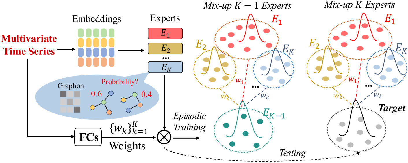
To prepare the system for this type of uncertainty, the framework's authors suggest using episodic learning. The essence of this approach lies in dividing the experts' functions. When an observation xi ∈ Ti is received as input, only the graphon Pi assigned to that time interval performs the main forecasting task. It is used to construct the graph Gi ⁓ Pi, which is then fed into the ST-GNN module to generate a forecast.

Thus, it is its own expert that is trained via the main loss function, which is responsible for forecasting accuracy.
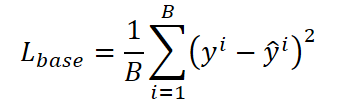
But the training process does not end there. The remaining experts {Pk}Kk=1,k≠i, although not used for direct forecasting in this case, play an important supporting role. They are used to form a graphon mixture Pimix(x), which should reproduce the structure of the reference graphon Pi as accurately as possible.
For this purpose, a gating network is introduced, which computes a vector of weights from the input signal xi.

These weights determine the proportions in which the other experts are combined.
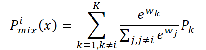
It is then compared with the reference graphon Pi.
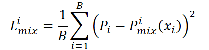
It is important to note that Lmix updates only the mixing weights w, without affecting the parameters of the graphons themselves. As a result, the experts retain their independence and continue to specialize in their respective market regimes, while the weight vector learns to combine them correctly in order to reproduce the properties of the reference graphon.
Thus, learning is divided into two parallel processes. Each expert refines its forecasting ability specifically within its own market regime, without interfering with the others, while the gating network is trained on an imitation task. It must learn to combine the knowledge of the other experts so that, together, they reproduce the structure of the current reference. This division of roles makes the model both highly specialized and flexible, capable of adapting to new market conditions.
This can be compared to the work of a team of analysts. Each of them has their own area of expertise. One has a better understanding of commodity assets, another specializes in currency markets, and a third specializes in bonds. When a new situation arises, the forecast is made by the analyst whose area of expertise is most relevant. At that moment, the others play a supporting role. They help the team better assess the extent to which their combined perspectives can replicate the lead expert's key insights.
After training, when the model is exposed to real-world market data, it finds itself in a situation of complete uncertainty for the first time. If, during training, it always had access to the correct graphon Pi assigned to the corresponding time interval, it no longer has such a cue. This corresponds to the natural situation in trading. A trader can rely on historical patterns, but can never know in advance exactly which phase of the cycle the market is in today.
The first step in the inference phase is for all experts to simultaneously generate a set of probabilistic graphons. Each of them develops its own interpretation of the structure of relationships between assets. Essentially, each expert puts forward its own market hypothesis. Some experts identify clearly defined sectoral clusters, while others capture global correlations between currencies and commodity assets, and still others detect unstable but meaningful local interrelationships.
The next step is to calculate the weight vector based on the current market signal xtest.

These weights reflect the importance of each expert at this moment. You could say that the gating network acts as an arbiter that determines the importance of each expert's opinion at that particular moment. If, for example, the market experiences a surge in volatility in commodity assets, experts trained on relevant scenarios will be given greater weight.
After the weights are calculated, a final mixed graphon is generated, providing an aggregated view of market relationships.
The key difference between the inference phase and the training phase is that all experts are now involved in the process at the same time. Whereas the system used to know which expert was the right one and used the others only for imitation, it now has to rely on a collective assessment. This point is of fundamental importance. The real market does not provide ready-made reference standards, and the model must be able to synthesize a new representation from accumulated knowledge.
In the final stage, a specific graph is sampled from the resulting probability matrix, reflecting the current distribution of relationships among assets. This graph is what is used in the ST-GNN module to generate a forecast. Here, the system essentially builds a forecast of market dynamics based not on a rigidly fixed structure, but on a flexibly formed representation created jointly by all the experts.
The result is a model that behaves like an experienced portfolio manager during the inference phase. It does not rely on a single source of information, but rather compares and combines different perspectives to create a dynamic market map. This approach makes it robust, flexible, and capable of maintaining forecasting accuracy even when familiar market patterns break down under the pressure of new events.
Another key advantage of the proposed approach lies in the versatility of the trainable graphons. Although they are used in conjunction with spatiotemporal graph neural networks (ST-GNNs) in the description above, their potential is much broader. Graphons are, in and of themselves, a flexible tool for describing probabilistic relationships and can serve as a connecting link for a wide range of architectures.
In particular, in transformer models, the graphon can act as a dynamic mask or a generated attention matrix, where the connections between elements in a sequence are determined not by predefined rules, but by a learned probabilistic structure. This paves the way for the creation of more adaptive transformers that are better able to capture changing market patterns. Furthermore, graphons can also be used in hybrid systems that combine CNNs, RNNs, and attention mechanisms, thereby improving the performance of any of these components.
The author's visualization of the ST-Expert framework is shown below.
Implementation Using MQL5
After reviewing the theoretical aspects of the ST-Expert framework, we move on to the practical implementation of its approaches using MQL5. And, of course, we will start our work by constructing graphons. But first, let's discuss the approaches we're taking in our implementation.
Personally, there are two aspects of the training process proposed by the authors of the framework that give me pause. The first is the need to preprocess the training sample to identify specific market regimes. This process is quite labor-intensive, requires an additional optimization step, and often relies on heuristics. In real market conditions, such strict segmentation may prove not only resource-intensive but also not entirely reliable. The boundaries between these market regimes are often blurred, and the regimes themselves can change rapidly. If we segment the historical data too rigidly, we risk losing important transitional phases, which are precisely what form the basis of many market movements.
The second point relates to the very logic of training graphons and weights. In the original formulation, it is assumed that when an observation from interval Ti is fed in, the corresponding expert Pi makes the prediction, while the remaining experts are combined into a mixture intended to reproduce its structure. Formally speaking, this approach looks elegant. Each graphon learns to predict its own market regime, while the gating network learns to combine the rest so that they can imitate the reference graphon. However, in practice, this raises a subtle problem. In effect, we rigidly fix the roles of the experts and rule out cross-training between them. This leads to the risk of over-specialization, where an expert performs genuinely well only within its narrow niche but is completely at a loss at the slightest shift in the market context.
Moreover, this approach makes the training of the weights dependent on the correctness of the reference graphon. If, at some point, Pi turns out to be corrupted by noise or captures an atypical market state, then the gating network will be forced to learn to reproduce it, rather than identify a more general pattern. In financial data, which is saturated with random outliers and spurious correlations, this can become a serious source of errors.
In our implementation, we will try to relax this rigid hierarchy. Instead of permanently assigning its own market regime to each expert, let us allow each graphon to contribute to the forecast with a probability that depends on the current state of the market. Formally, the system consists of N experts, and each expert provides its own forecast. Gating is a lightweight network that returns logits based on market features. To introduce episodicity and prevent any single expert from monopolizing attention, we use a random Dropout mask and pass the output through SoftMax. As a result, we obtain the weights and the ensemble’s final forecast. This approach allows the weights to learn not only from the task of imitating the reference, but also from collectively improving the forecast — where an expert’s importance is determined by the extent to which its contribution improves the ensemble in a given market state.
The loss function is constructed as a mixture of tasks. It should be based on a measure of the ensemble’s quality, with a weighted sum of the experts’ individual losses added to it. This encourages experts to improve their forecasts precisely where they matter most.
Dropout in the gating module turns training into an episodic trial. In each batch, the active set of experts changes slightly, and the model learns not to rely constantly on a single lucky expert. Dropout is enabled during training but disabled during inference, which allows the knowledge of all experts to be utilized.
The new CNeuronGraphons class serves as a domain-specific wrapper for our implementation of a flexible graphon ensemble. It encapsulates the gate state, the input data embeddings, the expert parameters, and the set of graphons itself — everything needed to generate a weighted graphon from a set of expert votes at each step.
class CNeuronGraphons   :  public CNeuronBaseOCL
  {
protected:
   CLayer            acProbability;
   CLayer            acDataEmb;
   CParams           cExpertsEmb;
   CNeuronBaseOCL    cGraphs;
   //---
   virtual bool      feedForward(CNeuronBaseOCL *NeuronOCL) override;
   virtual bool      updateInputWeights(CNeuronBaseOCL *NeuronOCL) override;
   virtual bool      calcInputGradients(CNeuronBaseOCL *NeuronOCL) override;

public:
                     CNeuronGraphons(void) {};
                    ~CNeuronGraphons(void) {};
   virtual bool      Init(uint numOutputs, uint myIndex, COpenCLMy *open_cl,
                          uint units, uint window, uint emb_dimension,
                          uint experts, float dropout,
                          ENUM_OPTIMIZATION optimization_type, uint batch);
   //---
   virtual int       Type(void) override const   {  return defNeuronGraphons;   }
   //--- methods for working with files
   virtual bool      Save(int const file_handle) override;
   virtual bool      Load(int const file_handle) override;
   //---
   virtual bool      WeightsUpdate(CNeuronBaseOCL *source, float tau) override;
   virtual void      SetOpenCL(COpenCLMy *obj) override;
   virtual void      SetActivationFunction(ENUM_ACTIVATION value) override { };
   virtual void      TrainMode(bool flag) override;
  };
Four internal objects are declared within the class, and each of them performs a distinct function — we will discuss the details when implementing the methods. In this implementation, their lifecycle is managed within the class, allowing the constructor and destructor to remain empty. No additional initialization or cleanup is required each time an object is created. This approach simplifies resource management, reduces overhead associated with creating multiple instances, and makes the class's behavior more predictable.
Initialization via `Init` provides full control over the configuration: the number of outputs, the neuron index in the network, a pointer to the OpenCL context, the number of internal units and the aggregation window, the embedding size, the number of experts, the dropout value, the optimization type, and the batch size. This makes it possible, on the one hand, to set up a lightweight MLP implementation of the gate for quick tests and, on the other hand, to switch to a high-performance OpenCL path when necessary. The `TrainMode(bool)` method controls the operating mode: during training, inverted Dropout is enabled and additional stochastic techniques may be used; during inference, disabling Dropout makes the behavior deterministic, which is important for production and stable trading decisions.
The entire process of creating the object's architecture and populating its internal components is handled by the Init method, which acts as the orchestrator of the entire process. It builds the basic neuron hierarchy, links the internal components to the OpenCL context, and carefully checks each step to produce a module that is fully ready for use.
bool CNeuronGraphons::Init(uint numOutputs, uint myIndex, COpenCLMy *open_cl,
                           uint units, uint window, uint emb_dimension,
                           uint experts, float dropout,
                           ENUM_OPTIMIZATION optimization_type, uint batch)
  {
   if(!CNeuronBaseOCL::Init(numOutputs, myIndex, open_cl, units * units, optimization_type, batch))
      return false;
   activation = None;
First, the method of the same name in the parent class is called — this is a required preliminary initialization of the base object. If it returns false, it means the base infrastructure is not ready and continuing the build is pointless, so the method immediately exits with a result of false. After a successful return, we explicitly clear the activation, since we will set the specific activation functions for the subcomponents individually below.
The next step is to initialize the cGraphs buffer — here we prepare a container for storing our experts' individual graphons. After that, the SIGMOID activation function is explicitly set so that the internal logic operates within the desired range.
   int index = 0;
   if(!cGraphs.Init(0, index, OpenCL, Neurons()*experts, optimization, iBatch))
      return false;
   cGraphs.SetActivationFunction(SIGMOID);
Next, a set of local variables is declared to temporarily store pointers to the subcomponents that we will manipulate during the step-by-step assembly of the model.
   CNeuronBaseOCL       *neuron  = NULL;
   CNeuronConvOCL       *conv    = NULL;
   CNeuronTransposeOCL  *transp  = NULL;
   CNeuronDropoutOCL    *dout    = NULL;
   CNeuronSoftMaxOCL    *softmax = NULL;
We now move on to building the model for generating expert usage probabilities. First, we clear the corresponding dynamic array and bind it to the OpenCL context.
//--- Probability
   acProbability.Clear();
   acProbability.SetOpenCL(OpenCL);
   index++;
   conv = new CNeuronConvOCL();
   if(!conv ||
      !conv.Init(experts, index, OpenCL, window, window, experts, units, 1, optimization, iBatch) ||
      !acProbability.Add(conv))
     {
      DeleteObj(conv);
      return false;
     }
   conv.SetActivationFunction(SoftPlus);
And we start the sequential assembly. First, we create a convolutional layer with the SoftPlus nonlinearity, which provides a smooth, monotonically increasing transformation of the logits before the next layer. After that, we create a fully connected layer that returns experts values — the very vector of logits before Dropout.
   index++;
   neuron = new CNeuronBaseOCL();
   if(!neuron ||
      !neuron.Init(0, index, OpenCL, experts, optimization, iBatch) ||
      !acProbability.Add(neuron))
     {
      DeleteObj(neuron);
      return false;
     }
As before, if an allocation or initialization error occurs, we correctly delete the object and terminate initialization with false.
Next, we create a Dropout layer — this is the object that implements the random dropping of experts mentioned earlier.
   index++;
   dout = new CNeuronDropoutOCL();
   if(!dout ||
      !dout.Init(0, index, OpenCL, experts, dropout, optimization, iBatch) ||
      !acProbability.Add(dout))
     {
      DeleteObj(dout);
      return false;
     }
The next step is to create a SoftMax layer, which converts the logits obtained earlier into a vector of expert importance probabilities.
   index++;
   softmax = new CNeuronSoftMaxOCL();
   if(!softmax ||
      !softmax.Init(0, index, OpenCL, experts, optimization, iBatch) ||
      !acProbability.Add(softmax))
     {
      DeleteObj(softmax);
      return false;
     }
   softmax.SetHeads(1);
Next, preparation begins for the input data embedding block acDataEmb. We clear it, bind it to OpenCL, and then begin assembling it from convolutional layers in the same way. Here, we use a small MLP consisting of two consecutive convolutional layers with a SoftPlus nonlinearity between them.
//--- Data Embedding
   acDataEmb.Clear();
   acDataEmb.SetOpenCL(OpenCL);
   index++;
   conv = new CNeuronConvOCL();
   if(!conv ||
      !conv.Init(0, index, OpenCL, window, window, 2 * emb_dimension, units, 1, optimization,
                                                                                   iBatch) ||
      !acDataEmb.Add(conv))
     {
      DeleteObj(conv);
      return false;
     }
   conv.SetActivationFunction(SoftPlus);
   index++;
   conv = new CNeuronConvOCL();
   if(!conv ||
      !conv.Init(0, index, OpenCL, 2 * emb_dimension, 2 * emb_dimension, emb_dimension, units,
                                                                   1, optimization, iBatch) ||
      !acDataEmb.Add(conv))
     {
      DeleteObj(conv);
      return false;
     }
   conv.SetActivationFunction(None);
As the output of this MLP, we expect to obtain embeddings for each time step of the analyzed multimodal sequence. However, to generate graphons, we will need a transposed copy of this representation. Therefore, a data transposition layer is added next.
   index++;
   transp = new CNeuronTransposeOCL();
   if(!transp ||
      !transp.Init(0, index, OpenCL, units, emb_dimension, optimization, iBatch) ||
      !acDataEmb.Add(transp))
     {
      DeleteObj(transp);
      return false;
     }
   transp.SetActivationFunction((ENUM_ACTIVATION)conv.Activation());
Next, all that remains is to initialize the object for generating our experts' embeddings, cExpertsEmb. Here, space is prepared for their individual representations.
   index++;
   if(!cExpertsEmb.Init(0, index, OpenCL, units * emb_dimension * experts, optimization, iBatch))
      return false;
//---
   return true;
  }
Finally, if there are no errors, the method returns true, indicating that the object is fully initialized and ready for training.
In the method’s behavior, we see a clear design philosophy: first, a graphon container is prepared; then, a probability generation pipeline is built; the input data embedding is formed; and finally, the parameter space for the experts is allocated. This sequence ensures a logical build process that is convenient for debugging and subsequent integration with OpenCL.
The feedForward method implements the forward pass as a carefully defined signal factory. First, we store a pointer to the current signal source in a local variable and declare an additional variable to temporarily store a reference to the layer being processed.
bool CNeuronGraphons::feedForward(CNeuronBaseOCL *NeuronOCL)
  {
   CNeuronBaseOCL* prev = NeuronOCL;
   CNeuronBaseOCL* current = NULL;
Next comes a pass through the block that predicts the probabilities of using experts. In the loop, we iterate through all the subcomponents responsible for generating logits.
//--- Probability
   for(int i = 0; i < acProbability.Total(); i++)
     {
      current = acProbability[i];
      if(!current ||
         !current.FeedForward(prev))
         return false;
      prev = current;
     }
In each iteration, we take the next component and ask it to perform its own forward pass. If the component is missing, or if its FeedForward returns false, we immediately terminate the method with a result of false. This is a strict and reliable fail-fast policy that protects against incorrect pipeline assembly.
After the layer has been executed successfully, we move the pointer to the source data object. The next layer will receive the output of the current layer as its input. As a result of this loop, we obtain a ready vector of normalized probabilities.
Next, we reinitialize the source data pointer and iterate through the acDataEmb block using exactly the same pattern. This secondary linear pass forms embeddings of the source data.
//--- Data Embedding
   prev = NeuronOCL;
   for(int i = 0; i < acDataEmb.Total(); i++)
     {
      current = acDataEmb[i];
      if(!current ||
         !current.FeedForward(prev))
         return false;
      prev = current;
     }
Next comes a small but important branch: if we are in training mode, we call the method for generating expert embeddings. This means that the parameters or expert representations are updated only during the training run. In inference mode, we expect that cExpertsEmb already contains ready weights, so we skip this step to save time.
//--- Experts
   if(bTrain)
      if(!cExpertsEmb.FeedForward())
         return false;
Next comes the core algebra. We calculate the auxiliary dimensions of the object's architecture.
//--- Graphs
   uint units = (uint)MathSqrt((double)Neurons());
   uint emb_dim = acDataEmb[-1].Neurons() / units;
   uint experts = cExpertsEmb.Neurons() / acDataEmb[-1].Neurons();
These simple calculations ensure that the shapes are consistent before matrix multiplication. The first matrix multiplication constructs each expert's own graph matrix. The resulting cGraphs buffer neatly contains a sequence of such matrices for all experts.
   if(!MatMul(cExpertsEmb.getOutput(), current.getOutput(), cGraphs.getOutput(),
              units, emb_dim, units, experts, false))
      return false;
   if(cGraphs.Activation() != None)
      if(!Activation(cGraphs.getOutput(), cGraphs.getOutput(), cGraphs.Activation()))
         return false;
After obtaining the raw graphon matrices, the control nonlinearity is applied. Here, we apply the selected activation function to all elements of the output buffer. This is an important step for bringing the values into the required range and adding the desired nonlinearity.
The final reduction transforms a set of expert matrices and a probability vector into a single final weighted-graph tensor. In other words, we take the vector of normalized weights from the last acProbability layer and combine the matrices of all experts into a single weighted result.
//--- Result
   if(!MatMul(acProbability[-1].getOutput(), cGraphs.getOutput(), Output, 1, experts, units * units, 1, false))
      return false;
//---
   return true;
  }
If all steps are completed successfully, the method returns true, confirming that the forward pass has completed correctly.
The algorithm for the backward pass methods follows the same logic as the forward pass, but proceeds in the opposite direction. Error signals travel through all layers in reverse order; gradients are carefully accumulated and propagated from the outputs to the inputs, ensuring that all components are trained correctly. Since the structure fully mirrors the feedForward method and all steps can easily be traced through the sequence already discussed, there is no point in going into detail about each stage now. For a complete understanding and practical work with all methods of the class, the full code, including the backward pass, is provided in the attachment.
We have worked hard today, and now it is time to take a short break, let the information sink in, and organize itself in our minds. In the next article, we will continue the work we have started and take a detailed look at the practical application of graphons.
Conclusion
In this article, we took an in-depth look at the theoretical aspects of the ST-Expert framework, which combines the principles of flexible gating, collective learning, and adaptive aggregation. We examined how a combination of probability generation blocks, input data embeddings, and expert representations enables the creation of models that are robust to noise and uncertainty.
The practical section presents the architecture of the CNeuronGraphons class, which enables the construction and training of graphons. The methods described provide a solid foundation for subsequent practical application.
References
Programs used in the article
| # | Name | Type | Description |
|---|---|---|---|
| 1 | Study.mq5 | Expert Advisor (EA) | Expert Advisor for offline model training |
| 2 | StudyOnline.mq5 | Expert Advisor (EA) | Expert Advisor for online model training |
| 3 | Test.mq5 | Expert Advisor (EA) | Expert Advisor for model testing |
| 4 | Trajectory.mqh | Class library | Structure for describing the system state and model architecture |
| 5 | NeuroNet.mqh | Class library | Class library for building a neural network |
| 6 | NeuroNet.cl | Library | Code library for the OpenCL program |
Translated from Russian by MetaQuotes Ltd.
Original article: https://www.mql5.com/ru/articles/19595
Warning: All rights to these materials are reserved by MetaQuotes Ltd. Copying or reprinting of these materials in whole or in part is prohibited.
This article was written by a user of the site and reflects their personal views. MetaQuotes Ltd is not responsible for the accuracy of the information presented, nor for any consequences resulting from the use of the solutions, strategies or recommendations described.

 Trade Duration vs Profitability Scatter Plot Indicator in MQL5
 Building a Market Behavior Analyzer in MQL5
 Building Volatility Models in MQL5: Implementing the APARCH Volatility Process
 From Novice to Expert: Trading Multi-Symbol Basket

- Free trading apps
- Over 8,000 signals for copying
- Economic news for exploring financial markets
You agree to website policy and terms of use