

Neural Networks in Trading: Probabilistic Time Series Forecasting (Encoder)
 4 944
4 944
 0
0

Introduction
We continue our exploration of the K²VAE framework — an advanced architecture designed specifically for time series modeling under conditions of high uncertainty. This model is based on a synthesis of three key ideas: linear dynamics in latent space (via Koopman operators), adaptive error filtering (using KalmanNet), and probabilistic modeling (based on a variational autoencoder). This approach makes it possible to simultaneously take into account both the patterns in the data and the degree of confidence in those patterns.
The main advantage of K²VAE is not simply generating a forecast, but rather constructing a probability distribution of the system's future states. Unlike traditional models, which are limited to a single most likely scenario, this approach yields a range of possible outcomes. Moreover, the width of this range depends on the model's degree of confidence in the current state. This makes the framework particularly useful in fields where it is important to account for risks and uncertainty — for example, in financial forecasting, logistics, or the management of technical systems.
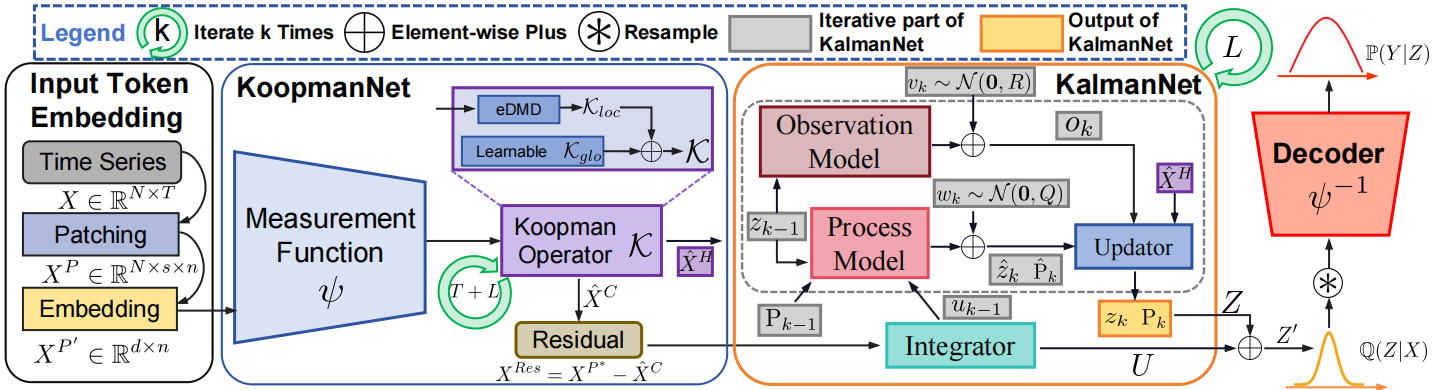
To understand how this flexibility and adaptability are achieved, let us examine the model's overall architecture. The K²VAE architecture can be broadly divided into three major components: Patching, the Encoder, and the Decoder, each of which performs its own role while being closely interconnected with the others.
- Patching prepares the input data and maps it to a latent representation.
- The Encoder is responsible for extracting the hidden state Z from the observed time series X. Unlike standard VAE models, this model uses a complex architecture that includes:
- KoopmanNet, a trainable counterpart of the Koopman operator that predicts the evolution of hidden features as a linear system;
- Attention Module, which analyzes the differences between reconstructed and actual values, making it possible to identify moments when the model diverges from reality;
- KalmanNet, a hybrid neural-network implementation of the Kalman filter that forms an uncertainty covariance matrix based on attention control signals;
- The VAE mechanism, which samples future tokens based on parameters provided by KalmanNet and KoopmanNet.
- The Decoder converts hidden variables back into observed variables, reconstructing the predicted values of the time series. At the same time, to preserve the probabilistic nature of the model, the Decoder is also implemented as a trainable neural network structure with two outputs: the mean and the variance. This allows us to fully model the distribution P(Y|Z) and account for the uncertainty in the forecast.
The author’s visualization of the K²VAE framework is shown below.
In the previous article, we focused on the groundwork: we implemented the basic infrastructure, ensured support for reusing trainable matrices, and laid the foundation for a robust and scalable architecture. General-purpose classes were created for generating parameters, the mechanism for updating them via standard backpropagation procedures was debugged, and a structure suitable for further component expansion was described. Thus, we have laid the foundation on which we can now build more complex modules.
The next logical step is to develop the Encoder, which performs a critical function: it transforms the original time series into a hidden latent representation suitable for linear analysis and probabilistic modeling. Moreover, this is achieved not through a simple set of layers, but through a carefully designed structure.
Discussion of Design Approaches
Before we begin the practical implementation of the Encoder using the MQL5 language, let’s take a detailed look at its architecture and design logic. This will help us not only properly navigate the work that follows, but also understand how each module contributes to the model’s overall behavior.
The Encoder used in the K²VAE framework is built according to a modular design and consists of four interconnected components, each of which performs a strictly defined function in the time-series processing workflow.
The first element in the processing chain is KoopmanNet — a neural-network interpretation of the Koopman operator, whose primary task is to approximate linear dynamics in a time series. It takes a hidden state as input and returns a prediction of the next state, assuming that the system’s behavior can be represented as a linear shift in some latent space. However, since real-world time series rarely follow a strictly linear trajectory, a projection into latent KoopmanNet space alone is not sufficient for reliable modeling. To enable the model not only to reproduce the trend but also to evaluate its own accuracy, the authors of the framework proposed a highly original mechanism.
In addition to predicting the next state, KoopmanNet is also trained to reconstruct transitions that have already occurred — in essence, to retrospectively reconstruct the trajectory from the previous values in the time series. Thus, the model is not limited to moving forward; it also looks back to verify how well its current parameters align with past observations. This bidirectional reasoning allows the model to calculate the difference between the predicted dynamics and the actual states of the system.
It is precisely this deviation (the difference between the transitions computed by KoopmanNet and the actual historical values) that serves as the basis for evaluating the quality of the linear approximation. Thus, the model gains the ability to self-diagnose and can dynamically adapt to changes or instabilities without losing touch with the linear structure that underlies it.
In the original implementation of the K²VAE framework, the KoopmanNet module consists of two separate, small fully connected models (MLPs), each of which models a different aspect of transitions in latent space: one is responsible for global dependencies, and the other for local dependencies. This approach makes perfect sense from a theoretical standpoint, but in practice it may prove to be overly rigid and limiting — especially when market data is volatile.
We propose enhancing KoopmanNet by using a more versatile and flexible sparse mixture of experts block — CNeuronTimeMoESparseExperts. This is a module from the TimeMoE framework that implements the Mixture of Experts (MoE) principle — a mechanism in which a set of specialized submodels (experts) operate in parallel, while a control mechanism selects the most appropriate one based on the input context.
The sparse mixture of experts block is not merely a technical implementation — it is the logical foundation for separating the local and global patterns present in financial time series. Two types of experts operate within this block. The first is a group of specialized local experts, each of which is responsible for identifying short-term transitions and context-dependent patterns. These experts essentially analyze market behavior over limited time intervals, adapting to current volatility and micro-trends.
The second is the global expert. It is built into the CNeuronTimeMoESparseExperts structure and acts as a generalized linear Koopman operator. Its purpose is to capture the stable, long-term dynamics of a time series by identifying the patterns that persist throughout the entire training window. In this way, the model gains a dual perspective on the data: detailed local analysis and a broad strategic perspective.
This architecture allows KoopmanNet not only to predict the next state, but also to reconstruct the preceding trajectory by retracing the series of transitions that led to the current state. Comparing the reconstructed transitions with the actual values allows the system to evaluate the accuracy of its own approximation.
Once KoopmanNet completes its reconstruction of the dynamics and predicts the next step, the Attention Module comes into play; its task is not simply to compare the actual and modeled values, but to analyze the deviations between them directly. Unlike the traditional cross-attention mechanism, which compares two data streams, this approach focuses exclusively on the error tensor, identifying recurring structures and patterns within it.
The authors of the K²VAE framework suggest viewing these deviations not as a byproduct, but as a full-fledged source of information. The idea is that the errors themselves contain a signal: they indicate where and to what extent KoopmanNet succeeds in describing the system, and which local features of the dynamics remain outside the scope of the linear model. Attention makes it possible to extract a tensor of control signals from these errors — a kind of instruction for adjusting the forecasts at the next stage.
Thus, rather than simply comparing predictions with actual results, the model learns to interpret its own weaknesses in a meaningful way. It is precisely this approach that underpins the high adaptability and intelligence of K²VAE, enabling it to operate effectively in a changing, unstable environment.
As part of the proposed implementation, we can use one of the Self-Attention modules already validated in practice and previously successfully applied to time series analysis. This not only significantly speeds up the development process but also ensures compatibility with the other components of the framework. This module can identify internal regularities in the structure of errors by detecting recurring patterns and local dependencies between deviations across different time intervals.
It is important to note that, in this context, Self-Attention is not used to process the original input sequence, as is typically done in standard transformers, but rather to analyze reconstruction errors that arise when reconstructing the dynamics in KoopmanNet. In effect, we shift the model's focus from the data itself to the result of its own work, allowing the system to evaluate itself from the outside and extract useful information from its errors.
However, an interesting nuance arises when implementing this approach. The depth of the history being analyzed and the planning horizon for which control signals are generated may differ in length. In the original version of the framework, this problem is solved using a linear projection — a compact transformation that allows the control vector to be adapted to the required planning horizon.
In our case, the situation is somewhat simpler. Since the model is designed to generate only a single next token, we do not need a sequence of control signals, but rather just a single vector. Of course, we could use the same linear projection. But we propose taking a different approach — and focusing on the last token's error in the context of the entire preceding chain of deviations.
This approach opens up new possibilities. Instead of treating an error as an isolated quantity, we analyze it in connection with the accumulated history of inaccuracies. This allows the attention mechanism to determine which specific segments of past dynamics had the greatest influence on the current error. The result is a control vector that does not merely respond to the current inaccuracy but reflects its causes, which are encoded in the system's previous states.
This method has a number of obvious advantages:
- Targeted attention: the model focuses on the error in the last step rather than distributing resources across the entire trajectory;
- Reduced computational load: there is no need to generate long vectors for each future step;
- Better interpretability: the control signal becomes meaningful and suitable for visual analysis and diagnostics.
Ultimately, we obtain a flexible internal control mechanism built into the Encoder, which allows the model to adapt to its own weaknesses and form the distribution for the next step more confidently via KalmanNet and VAE. This approach makes the architecture not only more robust but also noticeably more transparent in its behavior, which is particularly important when operating under market uncertainty.
The next component in the architecture of the Encoder is KalmanNet — a module that acts as an adaptive covariance matrix generator. Its task is not merely to pass information onward, but to actively assess the level of confidence in the linear forecast obtained from KoopmanNet. The control signal coming from the attention block serves as a kind of indicator of the reliability of the upstream model. If the deviations are small and persistent, KalmanNet interprets this as high confidence and, accordingly, tightens the covariance distribution — assuming that the subsequent behavior of the time series will, with high probability, follow the predicted scenario. However, if significant imbalance or structural shifts are observed in the errors, the model, on the contrary, expands the covariance matrix, opening up space for more variable, probabilistic outcomes.
Thus, KalmanNet effectively serves as a confidence indicator — a kind of barometer that reacts sensitively to turbulence within the data. It does not merely transmit signals; it interprets them, transforming imperceptible fluctuations into a mathematical form suitable for further use.
The operation of the Encoder is completed by the variational sampling block (VAE). It is here that the final latent representation of the future state is formed. However, the sampling is not performed blindly — it follows the logic established in the previous stages. The mean values are taken from KoopmanNet — as the basis for the predicted dynamics — while the degree of dispersion is specified by the covariance matrix generated by KalmanNet. As a result, we obtain not a point forecast but a probabilistic model that accounts for both the linear structure of the time series and the stochastic nature of the market.
This approach offers a clear strategic advantage. It allows the model to remain flexible under uncertainty, without fixating on a single development scenario, instead adapting its confidence to the context. This makes the framework particularly well suited for applications where dynamic decision-making based on risk and confidence assessments is more important than forecasting subsequent states.
In our implementation, to convey the degree of uncertainty and the level of potential risk, we do not limit ourselves to a single forecast. Instead, we sample a specified number of possible scenarios for how the time series may evolve at the next step. Each of these scenarios is a separate trajectory generated based on the common distribution formed by KoopmanNet and KalmanNet. This approach allows us not merely to obtain an averaged estimate, but to cover an entire spectrum of probable outcomes, thereby revealing how robustly the model anticipates the future.
Taken together, the interaction between KoopmanNet, the attention block, KalmanNet, and VAE forms a complex yet surprisingly logical structure, in which each component plays its own role in constructing a reliable and adaptive representation of the future.
Object Structure
After a detailed discussion of the architectural principles and the logic of component interaction within the Encoder of K²VAE, it is time to move on to examining its practical implementation. To ensure modularity, flexibility, and code readability, we have combined all key elements into a single object of the CNeuronK2VAEEncoder class, which inherits its core functionality from CNeuronBaseOCL.
This object incorporates everything needed for the full operational cycle of the Encoder — from analyzing the dynamics of time series using KoopmanNet, to constructing the covariance structure of future states in KalmanNet and sampling probabilistic forecasts via the VAE mechanism. The object includes specialized components such as the Koopman network, the attention block, and the Kalman filter, as well as technical layers for transformations, linear operations, and matrix computations.
Below is the structure of the CNeuronK2VAEEncoder class, with each component performing a specific function within the overall process of encoding the observed sequence. This implementation enables step-by-step analysis and debugging at any level of model depth, and also provides advanced scaling capabilities when working with various architectural configurations and different depths of analysis.
class CNeuronK2VAEEncoder   :  public CNeuronBaseOCL
  {
protected:
   //--- Koopman
   CNeuronTimeMoESparseExperts   cKoopman;
   CNeuronBaseOCL                cKoopmanPred;
   CNeuronBaseOCL                cKoopmanRest;
   //---
   CNeuronTimeMoEAttention       cAuxiliaryNet;
   //--- Kalman Filter
   CParams              cB;      // Control input matrix B
   CParams              cF;      // State transition matrix F
   CParams              cH;      // Observation matrix H
   CParams              cQ;      // Learnable covariance matrices Q
   CParams              cR;      // Learnable covariance matrices R
   CNeuronBaseOCL       cP;      // Covariance matrices P
   //---
   CNeuronTransposeOCL  cFT;
   CNeuronTransposeOCL  cHT;
   CNeuronTransposeOCL  cQT;
   CNeuronTransposeOCL  cRT;
   CNeuronTransposeOCL  cPT;
   //---
   CNeuronBaseOCL       cQ_QT;
   CNeuronBaseOCL       cR_RT;
   CNeuronBaseOCL       cXPred;
   CNeuronBaseOCL       cF_P;
   CNeuronBaseOCL       cPPred;
   //---
   CNeuronBaseOCL       cP_HT;
   CNeuronBaseOCL       cH_P_HT;
   matrix<double>       mS, mSGrad;
   CNeuronBaseOCL       cSInv;
   CNeuronBaseOCL       cK;
   CNeuronTransposeOCL  cKT;
   CNeuronBaseOCL       cYPred;
   CNeuronBaseOCL       cDeltY;
   CNeuronBaseOCL       cX;
   CNeuronBaseOCL       cK_H;
   CNeuronBaseOCL       cIdifK_H;
   CNeuronTransposeOCL  cIdifK_HT;
   matrix<double>       mP;
   matrix<double>       mPGrad;
   matrix<double>       mNoise;
   matrix<double>       mGrad;
   //---
   virtual bool      feedForward(CNeuronBaseOCL *NeuronOCL) override;
   virtual bool      updateInputWeights(CNeuronBaseOCL *NeuronOCL) override;
   virtual bool      calcInputGradients(CNeuronBaseOCL *NeuronOCL) override;

public:
                     CNeuronK2VAEEncoder(void) {};
                    ~CNeuronK2VAEEncoder(void) {};
   //---
   virtual bool      Init(uint numOutputs, uint myIndex, COpenCLMy *open_cl,
                          uint window, uint window_key, uint units_cross,
                          uint heads, uint layers, uint scenarios,
                          uint experts, uint experts_dimension, uint topK,
                          ENUM_OPTIMIZATION optimization_type, uint batch);
   //---
   virtual bool      Save(const int file_handle) override;
   virtual bool      Load(const int file_handle) override;
   //---
   virtual int       Type(void)        const                      {  return defNeuronK2VAEEncoder; }
   virtual void      TrainMode(bool flag) override;
   virtual void      SetOpenCL(COpenCLMy *obj);
   //---
   virtual bool      WeightsUpdate(CNeuronBaseOCL *source, float tau);
  };
In the structure of the new class presented here, special attention should be paid to the key components that reflect the logic of the entire Encoder architecture. A powerful CNeuronTimeMoESparseExperts module is used as KoopmanNet, combining the local flexibility of a sparse mixture of experts with the stability of a global predictor. This solution makes it possible to effectively model both short-term and persistent dynamics in time series.
CNeuronTimeMoEAttention is used as the Attention Module and is responsible for analyzing the structure of reconstruction errors. It identifies patterns in the deviations, forming control features for assessing confidence in KoopmanNet forecasts.
The Kalman filter block occupies a special place in the implementation. Here we see the trainable matrices B, F, H, Q, and R, each of which is represented as a separate instance of the CParams class. This approach not only allows centralized management of the filter parameters but also ensures that they can be fully adapted during training.
In addition to these components, the class structure also contains many auxiliary objects that ensure the correct implementation of the step-by-step logic of KalmanNet and enable efficient management of all tensor operations within the Encoder. The functionality of helper objects will be discussed in greater detail as we implement the class's methods.
The internal organization of the CNeuronK2VAEEncoder class assumes a static declaration of all components it uses. This solution simplifies the object's life cycle: we do not need to manually allocate and deallocate memory. Consequently, the class's constructor and destructor can remain empty, without burdening the code with unnecessary logic.
All architectural setup, including the configuration of KoopmanNet, the attention parameters, and the Kalman filter parameters, is handled entirely within the Init method. This is where the object takes on its concrete form: the attention parameters are configured, the dimensions of the control features are specified, and the number of experts, input window depth, and other critically important model characteristics are set.
bool CNeuronK2VAEEncoder::Init(uint numOutputs, uint myIndex, COpenCLMy * open_cl,
                               uint window, uint window_key, uint units_cross,
                               uint heads, uint layers, uint scenarios,
                               uint experts, uint experts_dimension, uint topK,
                               ENUM_OPTIMIZATION optimization_type, uint batch)
  {
   if(!CNeuronBaseOCL::Init(numOutputs, myIndex, open_cl, window * scenarios, optimization_type, batch))
      return false;
In the first stage, control is passed to the function of the same name in the base class. This makes it possible to use the already implemented mechanisms for basic validation of input parameters, as well as to initialize inherited interfaces and shared components. This approach ensures a uniform initialization standard for all neural layers, simplifying the maintenance and expansion of the architecture.
The issue of memory organization deserves special attention. Since, in our implementation, the K²VAE Encoder returns not a single vector but a set of possible future scenarios generated through sampling, the result buffer must be sized accordingly.
Next, we move on to initializing the KoopmanNet block, which in our implementation is represented by the CNeuronTimeMoESparseExperts module. We initialize the sparse mixture of experts module by specifying the number of models and their dimensionality. This component is responsible for extracting both local and global patterns from a time series by simulating the behavior of Koopman operators.
//--- Koopman
   int index = 0;
   if(!cKoopman.Init(0, index, OpenCL, window, 2 * window, units_cross, 1, experts, topK, optimization, iBatch))
      return false;
   index++;
   if(!cKoopmanPred.Init(0, index, OpenCL, window, optimization, iBatch))
      return false;
   index++;
   if(!cKoopmanRest.Init(0, index, OpenCL, window * (units_cross - 1), optimization, iBatch))
      return false;
Next, we initialize two helper objects: cKoopmanPred and cKoopmanRest. The first will be used to store the forecast values calculated by KoopmanNet, and the second will be used to reconstruct the already observed states of the time series.
The next step is to initialize the Attention Module, which in our implementation is represented by the cAuxiliaryNet object.
index++;
if(!cAuxiliaryNet.Init(0, index, OpenCL, window, window_key, 1, window, units_cross - 1,
                                                   heads, layers, optimization, iBatch))
   return false;
However, a key part of the new class internal architecture centers on the organization of the Kalman filter’s operation: this is where the bulk of the computations and the largest amount of logic implemented in the Init method are concentrated.
In the first step, we sequentially initialize the square matrices of the filter’s trainable parameters: the state transition matrices F, the control input matrices B, the observation matrices H, as well as the covariance matrices for model errors Q and observation errors R.
//--- Kalman Filter
   index++;
   if(!cB.Init(0, index, OpenCL, window * window, optimization, iBatch) ||
      !cB.Identity(window, window))
      return false;
   index++;
   if(!cF.Init(0, index, OpenCL, window * window, optimization, iBatch) ||
      !cF.Identity(window, window))
      return false;
   index++;
   if(!cH.Init(0, index, OpenCL, window * window, optimization, iBatch) ||
      !cH.Identity(window, window))
      return false;
   index++;
   if(!cQ.Init(0, index, OpenCL, window * window, optimization, iBatch) ||
      !cQ.Identity(window, window))
      return false;
   index++;
   if(!cR.Init(0, index, OpenCL, window * window, optimization, iBatch) ||
      !cR.Identity(window, window))
      return false;
   index++;
   if(!cP.Init(0, index, OpenCL, window * window, optimization, iBatch) ||
      !cP.getOutput().Fill(matrix<float>::Identity(window, window)))
      return false;
When each of these matrices is initialized, its dimensions are specified. Next, to ensure the numerical stability of the Kalman filter during the initial training iterations, all of these matrices are initialized with diagonal values. This initialization ensures that the covariance matrices are positive-definite and prevents instability in the calculations involved in the inversion of matrix S during the forecast correction process.
The diagonal initialization approach not only stabilizes the initial stages of training but also ensures that the model is uniformly sensitive to the various components of the latent state, which is critically important when working with time series in which dominant trends can mask weak but significant signals.
The next step is to prepare the objects responsible for transposing the corresponding matrices. This is an important and, at first glance, technical detail, but it is directly related to the proper operation of the entire algorithm. This is because, during the Kalman filter computations, we repeatedly need to refer not only to the matrices F, H, Q, R, and P themselves, but also to their transposed versions. To ensure this, we allocate and initialize the corresponding transpose objects in advance.
index++;
if(!cFT.Init(0, index, OpenCL, window, window, optimization, iBatch))
   return false;
index++;
if(!cHT.Init(0, index, OpenCL, window, window, optimization, iBatch))
   return false;
index++;
if(!cQT.Init(0, index, OpenCL, window, window, optimization, iBatch))
   return false;
index++;
if(!cRT.Init(0, index, OpenCL, window, window, optimization, iBatch))
   return false;
index++;
if(!cPT.Init(0, index, OpenCL, window, window, optimization, iBatch))
   return false;
Thus, a form of buffering for the transposed representations is implemented, which significantly speeds up computations and simplifies the code structure in the main part of the filtering algorithm. In addition, this enhances the modularity of the architecture, as it allows each filter element to be handled independently without disrupting the overall execution logic.
It is worth paying special attention to the noise covariance matrices: Q (process covariance) and R (observation covariance). For the Kalman filter algorithm to function correctly, these matrices must have two key properties: they must be symmetric about the main diagonal and positive-definite. Failure to satisfy these conditions may lead to unstable filtering, the appearance of imaginary values during matrix inversion, or complete degradation of the state estimate.
To ensure that these properties hold during training, we use a time-tested and widely used technique: we represent the matrices Q and R as the product of each matrix and its transpose. This representation automatically makes the resulting matrices symmetric and positive-definite, unless the original matrix is singular. This eliminates the need to manually monitor the diagonal entries or introduce regularization.
index++;
if(!cQ_QT.Init(0, index, OpenCL, window * window, optimization, iBatch))
   return false;
index++;
if(!cR_RT.Init(0, index, OpenCL, window * window, optimization, iBatch))
   return false;
The next step in configuring the Encoder is to initialize the objects used to store intermediate computational results. These objects play a key role in the step-by-step implementation of the Kalman filter algorithm, where each calculation is based on the results of previous operations. In addition, we will use these values during the backward pass to ensure that the error gradient is distributed correctly.
We begin by initializing the cXPred object, which will store the predicted state of the system before the correction step is applied.
index++;
if(!cXPred.Init(0, index, OpenCL, window, optimization, iBatch))
   return false;
index++;
if(!cF_P.Init(0, index, OpenCL, window * window, optimization, iBatch))
   return false;
index++;
if(!cPPred.Init(0, index, OpenCL, window * window, optimization, iBatch))
   return false;
Next, we initialize the objects cF_P and cPPred, which store, respectively, the product of the transition matrix and the covariance matrix, and the predicted covariance. These data are needed for subsequent operations that assess the reliability of the forecast.
Next, the cP_HT and cH_P_HT blocks are configured sequentially; they compute intermediate values when calculating the S matrix — the covariance of the observation prediction error.
   index++;
   if(!cP_HT.Init(0, index, OpenCL, window * window, optimization, iBatch))
      return false;
   index++;
   if(!cH_P_HT.Init(0, index, OpenCL, window * window, optimization, iBatch))
      return false;
//---
   mS = mSGrad = matrix<double>::Zeros(window, window);
At the same time, the matrices mS and mSGrad are created and initialized; they will be used to store the covariance values themselves and the corresponding gradients during training.
The cSInv object is intended to store the inverse of the S matrix, which is needed to compute the Kalman gain cK; the gain also has its own transpose, cKT.
   index++;
   if(!cSInv.Init(0, index, OpenCL, window * window, optimization, iBatch))
      return false;
   index++;
   if(!cK.Init(0, index, OpenCL, window * window, optimization, iBatch))
      return false;
   index++;
   if(!cKT.Init(0, index, OpenCL, window, window, optimization, iBatch))
      return false;
//---
   index++;
   if(!cYPred.Init(0, index, OpenCL, window, optimization, iBatch))
      return false;
//---
   index++;
   if(!cDeltY.Init(0, index, OpenCL, window, optimization, iBatch))
      return false;
Next, the cYPred block — which predicts observed values — and the cDeltY block — which represents the difference between the prediction and the actual observation — are initialized.
Special attention is given to the cX object, which stores the final, corrected state after the Kalman filter has been applied.
   index++;
   if(!cX.Init(0, index, OpenCL, window, optimization, iBatch))
      return false;
//---
   index++;
   if(!cK_H.Init(0, index, OpenCL, window * window, optimization, iBatch))
      return false;
//---
   index++;
   if(!cIdifK_H.Init(0, index, OpenCL, window * window, optimization, iBatch))
      return false;
//---
   index++;
   if(!cIdifK_HT.Init(0, index, OpenCL, window, window, optimization, iBatch))
      return false;
These are followed by cK_H, cIdifK_H, and cIdifK_HT, which are designed to record the results of the mathematical transformations required for correct error backpropagation and the updating of covariance estimates.
Finally, we initialize the matrices mP and mPGrad, as well as the auxiliary arrays mNoise and mGrad, which will be used to generate noise during the sampling phase and to compute gradients during model training.
   mP = mPGrad = mS;
   mNoise = mGrad = matrix<double>::Zeros(scenarios, window);
//---
   return true;
  }
Thus, at this stage, a fully fledged computational infrastructure is being created to ensure the stable and correct operation of the Kalman filter within the Encoder of K²VAE. After successfully initializing all internal components, the initialization method completes, returning a boolean result indicating the outcome of the operations to the calling program.
Organization of the Forward Pass
Moving from the stage of initializing storage objects to the description of the forward pass method feedForward, we effectively delve into the depths of the computational logic of the Encoder of K²VAE. This is where all the previously prepared components are integrated into a single system. The entire structure, like a well-coordinated mechanism, begins operating, transforming the initial observations into internal representations.
The forward pass begins with the Koopman block — a key component of the model that learns the system's linear dynamics during training. During inference, as part of the forward pass, this module generates a series of reconstructions and a single predicted state based on the sequence being analyzed and the previously learned linear structure of changes. Thus, its output consists of two important components: first, a prediction of the future state, which is based exclusively on the most recent observation and the linear patterns that have been learned; and second, a reconstruction of the entire sequence of previous states, extending back to the depth of the historical data analysis.
bool CNeuronK2VAEEncoder::feedForward(CNeuronBaseOCL * NeuronOCL)
  {
//--- Koopman
   if(!cKoopman.FeedForward(NeuronOCL))
      return false;
//--- Pred / Rest
   if(!DeConcat(cKoopmanPred.getOutput(), cKoopmanRest.getPrevOutput(), cKoopman.getOutput(),
                cKoopman.GetWindow(), cKoopman.Neurons() - cKoopman.GetWindow(), 1))
      return false;
   if(!Different(NeuronOCL.getOutput(), cKoopmanRest.getPrevOutput(),
                 cKoopmanRest.getOutput(), cKoopman.GetWindow()))
      return false;
This separation is particularly important: the forecast is used in the Kalman filter block, while the residual sequence (the difference between the actual data and its reconstruction) is passed to the Attention Module, which processes those aspects of the dynamics that do not fit into the linear model.
//--- Rest Attention
   if(!cAuxiliaryNet.FeedForward(cKoopmanRest.AsObject()))
      return false;
Next, if the model is operating in training mode, all trainable components of the Kalman filter are activated. These are the state-transition, control-input, and observation matrices, as well as the covariance matrices for model and measurement errors.
//--- Kalman Filter
   if(bTrain)
     {
      if(!cB.FeedForward())
         return false;
      if(!cF.FeedForward())
         return false;
      if(!cH.FeedForward())
         return false;
      if(!cQ.FeedForward())
         return false;
      if(!cR.FeedForward())
         return false;
      if(!cFT.FeedForward(cF.AsObject()))
         return false;
      if(!cHT.FeedForward(cH.AsObject()))
         return false;
      if(!cQT.FeedForward(cQ.AsObject()))
         return false;
      if(!cRT.FeedForward(cR.AsObject()))
         return false;
Since the matrices Q and R must be positive-definite for the filter to operate correctly, they are first stabilized by multiplying them by their own transposes.
 if(!MatMul(cQ.getOutput(), cQT.getOutput(), cQ_QT.getOutput(),
            cQT.GetCount(), cQT.GetWindow(), cQT.GetCount(), 1, true))
    return false;
 if(!MatMul(cR.getOutput(), cRT.getOutput(), cR_RT.getOutput(),
            cRT.GetCount(), cRT.GetWindow(), cRT.GetCount(), 1, true))
    return false;
}
Once all the parameters have been prepared, the prediction stage begins. First, the state prediction for the next step is computed by combining two information streams — the input data and the output of the attention module. These vectors are projected using the trainable parameter matrices F and B, and are then added together. As a result, the intermediate state XPred is formed.
//--- Prediction step
   if(!MatMul(NeuronOCL.getOutput(), cFT.getOutput(), cXPred.getGradient(),
              1, cFT.GetWindow(), cFT.GetCount(), 1, true))
      return false;
   if(!MatMul(cAuxiliaryNet.getOutput(), cB.getOutput(), cXPred.getPrevOutput(),
              1, cFT.GetWindow(), cFT.GetCount(), 1, true))
      return false;
   if(!SumAndNormilize(cXPred.getGradient(), cXPred.getPrevOutput(), cXPred.getOutput(),
                       cFT.GetCount(), false, 0, 0, 0, 1))
      return false;
Next, the predicted covariance of the state error is calculated. To do this, the transition matrix and the current covariance matrix are multiplied in sequence, and then the model noise matrix Q is added, thereby generating the predicted covariance P_pred.
if(!MatMul(cF.getOutput(), cP.getOutput(), cF_P.getOutput(),
           cFT.GetCount(), cFT.GetWindow(), cP.Neurons() / cFT.GetWindow(), 1, true))
   return false;
if(!MatMul(cF_P.getOutput(), cFT.getOutput(), cPPred.getOutput(),
           cFT.GetCount(), cFT.GetWindow(), cFT.GetCount(), 1, true))
   return false;
if(!SumAndNormilize(cPPred.getOutput(), cQ_QT.getOutput(), cPPred.getOutput(),
                    cHT.GetWindow(), false, 0, 0, 0, 1))
   return false;
At this stage, the forecast adjustment begins — which is what makes the Kalman filter so highly valued. First, the covariance of the measurement error is calculated, and a matrix S is formed, representing the sum of the observed variance and the predicted variance.
//--- Update step
   if(!MatMul(cPPred.getOutput(), cHT.getOutput(), cP_HT.getOutput(),
              cPPred.Neurons() / cHT.GetWindow(), cHT.GetWindow(), cHT.GetCount(), 1, true))
      return false;
   if(!MatMul(cH.getOutput(), cP_HT.getOutput(), cH_P_HT.getOutput(),
              cHT.GetCount(), cHT.GetWindow(), cHT.GetCount(), 1, true))
      return false;
   if(!SumAndNormilize(cH_P_HT.getOutput(), cR_RT.getOutput(), cR_RT.getPrevOutput(),
                       cRT.GetWindow(), false, 0, 0, 0, 1))
      return false;
To compute the Kalman gain K, which acts as a weighting coefficient in state correction, the inverse of matrix S is used. We decided not to build a matrix inversion algorithm from scratch. Instead, we used the existing matrix-operation functionality in MQL5. If necessary, the matrix is stabilized, diagonalized, and reconstructed to avoid singularity.
if(cR_RT.getPrevOutput().GetData(mSGrad) <= 0)
   return false;
mS = mSGrad.Inv();
if(mS.Rows() == 0)
  {
   mSGrad = mSGrad + mSGrad.Transpose();
   vector<double> eigvals;
   matrix<double> eigvecs;
   if(!mSGrad.Eig(eigvecs, eigvals))
      return false;
   if(eigvals.Size() > 0)
     {
      if(!eigvals.Clip(1e-6, DBL_MAX))
         return false;
      mSGrad = matrix<double>::Zeros(eigvals.Size(), eigvals.Size());
      mSGrad.Diag(eigvals);
      mSGrad = eigvecs.MatMul(mSGrad.MatMul(eigvecs.Transpose()));
      mSGrad = mSGrad + mSGrad.Transpose();
      mS = mSGrad.Inv();
     }
   if(mS.Rows() == 0)
     {
      mSGrad.Identity();
      mS = mSGrad;
     }
  }
cSInv.getOutput().Fill(mS);
if(!MatMul(cP_HT.getOutput(), cSInv.getOutput(), cK.getOutput(),
           cHT.GetCount(), (int)mS.Rows(), (int)mS.Cols(), 1, true))
   return false;
During the measurement update phase, the model adjusts the previously predicted state based not on actual observations, but on an alternative prediction obtained from KoopmanNet. First, the expected value of the observation is calculated by multiplying the predicted state XPred by the transposed observation matrix H. This value (YPred) reflects what the observation would be if the model were to make no errors in its prediction.
//--- Measurement update
   if(!MatMul(cXPred.getOutput(), cHT.getOutput(), cYPred.getOutput(),
              1, cHT.GetWindow(), cHT.GetCount(), 1, true))
      return false;
   if(!Different(cKoopmanPred.getOutput(), cYPred.getOutput(), cDeltY.getOutput(),
                 1, 0, 0, 0, 1))
      return false;
   if(!MatMul(cDeltY.getOutput(), cK.getOutput(), cX.getPrevOutput(), 1,
              cDeltY.Neurons(), cX.Neurons(), 1, true))
      return false;
   if(!SumAndNormilize(cX.getPrevOutput(), cXPred.getOutput(), cX.getOutput(), 1, false, 0, 0, 0, 1))
      return false;
The difference between the predictions of the two models is interpreted as an error. By multiplying this error by the Kalman gain K, we obtain a correction vector that is added to the initial forecast XPred, resulting in the corrected state X.
At the same time, the state covariance matrix P is updated using the Joseph stabilized form, which helps prevent the accumulation of numerical errors and preserve symmetry.
//--- Joseph stabilized form for P
   if(!MatMul(cK.getOutput(), cH.getOutput(), cK_H.getOutput(), cKT.GetCount(),
              cKT.GetWindow(), cHT.GetWindow(), 1, true))
      return false;
   if(!IdentDifferent(cK_H.getOutput(), cIdifK_H.getOutput(), cHT.GetWindow(), 0, 0, 1))
      return false;
   if(!cIdifK_HT.FeedForward(cIdifK_H.AsObject()))
      return false;
   if(!cKT.FeedForward(cK.AsObject()))
      return false;
   if(!MatMul(cIdifK_H.getOutput(), cPPred.getOutput(), cIdifK_H.getPrevOutput(),
              cIdifK_HT.GetCount(), cIdifK_HT.GetWindow(), cIdifK_HT.GetWindow(), 1, true))
      return false;
   if(!MatMul(cIdifK_H.getPrevOutput(), cIdifK_HT.getOutput(), cP.getPrevOutput(),
              cIdifK_HT.GetCount(), cIdifK_HT.GetWindow(), cIdifK_HT.GetCount(), 1, true))
      return false;
   if(!MatMul(cK.getOutput(), cR_RT.getOutput(), cK.getPrevOutput(),
              cKT.GetCount(), cRT.GetCount(), cRT.GetCount(), 1, true))
      return false;
   if(!MatMul(cK.getPrevOutput(), cKT.getOutput(), cKT.getPrevOutput(),
              cKT.GetCount(), cKT.GetWindow(), cKT.GetCount(), 1, true))
      return false;
   if(!SumAndNormilize(cP.getPrevOutput(), cKT.getPrevOutput(), cP.getOutput(), cPT.GetWindow(), false, 0, 0, 0, 1))
      return false;
   if(!cPT.FeedForward(cP.AsObject()))
      return false;
   if(!SumAndNormilize(cP.getOutput(), cPT.getOutput(), cP.getOutput(), 1, false, 0, 0, 0, 0.5f))
      return false;
Once all calculations are complete, the final step is to generate the output vector. To do this, sampling is performed based on the obtained inverse covariance matrix P⁻¹. Random noise is scaled by P, and the result is added to the state vector X, forming the final representation.
   if(!SumAndNormilize(cX.getOutput(), cAuxiliaryNet.getOutput(), cX.getOutput(), 1, false, 0, 0, 0, 1))
      return false;
//--- Sample Output
   if(!cP.getOutput().GetData(mPGrad))
      return false;
   if(mPGrad.HasNan() > 0)
     {
      mPGrad.Identity();
      if(!cP.getOutput().Fill(mPGrad))
         return false;
     }
   mP = mPGrad.Inv();
   if(mP.Rows() == 0)
     {
      mPGrad = mPGrad + mPGrad.Transpose();
      vector<double> eigvals;
      matrix<double> eigvecs;
      if(!mPGrad.Eig(eigvecs, eigvals))
         return false;
      if(eigvals.Size() > 0)
        {
         if(!eigvals.Clip(1e-6, DBL_MAX))
            return false;
         mPGrad = matrix<double>::Zeros(eigvals.Size(), eigvals.Size());
         mPGrad.Diag(eigvals);
         mPGrad = eigvecs.MatMul(mPGrad.MatMul(eigvecs.Transpose()));
         mPGrad = mPGrad + mPGrad.Transpose();
         mP = mPGrad.Inv();
        }
      if(mP.Rows() == 0)
        {
         mPGrad.Identity();
         if(!cP.getOutput().Fill(mPGrad))
            return false;
         mP = mPGrad.Inv();
        }
     }
   mNoise.Random(-1, 1);
   matrix<double> temp = mNoise.MatMul(mP);
   if(!PrevOutput.Fill(temp))
      return false;
   if(!SumVecMatrix(cX.getOutput(), PrevOutput, Output, (int)mNoise.Cols(), 0, 0, 0, 1))
      return false;
//---
   return true;
  }
It is worth emphasizing that the final stage of generating the results tensor is not limited to constructing a single scenario. Instead, the model generates a whole range of possible trajectories, each of which is a realization from a multivariate distribution described by the covariance matrix P. This is not just an elegant mathematical trick, but rather reflects the model's degree of confidence in its own forecast.
It is precisely this approach that makes the model particularly valuable in conditions of market instability or a lack of reliable information: it can do more than simply predict a single possible future scenario; it can outline an entire bundle of possible trajectories informed by training. This transforms the feedForward output into a probabilistic cloud of solutions. Each of them reflects different aspects of how events might unfold.
Characteristics of the Error Gradient Distribution
Once the model has generated a range of possible trajectories, the forward pass phase ends and an equally important stage begins: backpropagation of the error gradient. We implement it in the calcInputGradients method, whose main task is to pass gradients from the model output level to the input data, correctly propagating the error through all related components.
The algorithm begins by distributing the gradient between the mean forecast values of the linear model and the covariance matrix P.
bool CNeuronK2VAEEncoder::calcInputGradients(CNeuronBaseOCL *NeuronOCL)
  {
   if(!NeuronOCL)
      return false;
//--- From Output
   if(!SumVecMatrixGrad(cX.getGradient(), PrevOutput, Gradient, (int)mNoise.Cols(), 0, 0, 0, 1))
      return false;
   if(!PrevOutput.GetData(mGrad))
      return false;
   mPGrad = mNoise.Transpose().MatMul(mGrad);
   mP = mP.Transpose();
   mP = (mP * (-1)).MatMul(mPGrad.MatMul(mP));
We will also pass the error gradient through the Joseph stabilized form.
//--- Joseph stabilized form for P
   if(!cPT.getGradient().Fill(mP))
      return false;
   if(!cP.CalcHiddenGradients(cPT.AsObject()))
      return false;
   if(!SumAndNormilize(cP.getGradient(), cPT.getGradient(), cP.getGradient(), 1, false, 0, 0, 0, 0.5f))
      return false;
//---
   if(!MatMulGrad(cK.getPrevOutput(), cKT.getPrevOutput(),
                  cKT.getOutput(), cKT.getGradient(),
                  cP.getGradient(), cKT.GetCount(),
                  cKT.GetWindow(), cKT.GetCount(), 1, true))
      return false;
   if(!MatMulGrad(cK.getOutput(), cK.getPrevOutput(),
                  cR_RT.getOutput(), cR_RT.getGradient(),
                  cKT.getPrevOutput(), cKT.GetCount(),
                  cRT.GetCount(), cRT.GetCount(), 1, true))
      return false;
   if(!MatMulGrad(cIdifK_H.getPrevOutput(), cIdifK_HT.getPrevOutput(),
                  cIdifK_HT.getOutput(), cIdifK_HT.getGradient(),
                  cP.getGradient(), cIdifK_HT.GetCount(),
                  cIdifK_HT.GetWindow(), cIdifK_HT.GetCount(), 1, true))
      return false;
   if(!MatMulGrad(cIdifK_H.getOutput(), cIdifK_H.getPrevOutput(),
                  cPPred.getOutput(), cPPred.getGradient(),
                  cIdifK_HT.getPrevOutput(), cIdifK_HT.GetCount(),
                  cIdifK_HT.GetWindow(), cIdifK_HT.GetWindow(), 1, true))
      return false;
//---
   if(!cK.CalcHiddenGradients(cKT.AsObject()))
      return false;
   if(!SumAndNormilize(cK.getGradient(), cK.getPrevOutput(), cK.getGradient(), 1, false, 0, 0, 0, 1))
      return false;
The resulting matrix is passed on and initializes the gradient response chain in the Kalman filter block. First, through the measurement update module.
//--- Measurement update
   if(!cIdifK_H.CalcHiddenGradients(cIdifK_HT.AsObject()))
      return false;
   if(!SumAndNormilize(cIdifK_H.getGradient(), cIdifK_H.getPrevOutput(), cIdifK_H.getGradient(),
                                                                          1, false, 0, 0, 0, 1))
      return false;
   if(!IdentDifferentGrad(cK_H.getGradient(), cIdifK_H.getGradient(), cHT.GetWindow(), 0, 0, 1))
      return false;
   if(!MatMulGrad(cK.getOutput(), cK.getPrevOutput(),
                  cH.getOutput(), cH.getGradient(),
                  cK_H.getGradient(), cKT.GetCount(),
                  cKT.GetWindow(), cHT.GetWindow(), 1, true))
      return false;
//---
   if(!MatMulGrad(cDeltY.getOutput(), cDeltY.getGradient(),
                  cK.getOutput(), cK.getPrevOutput(),
                  cX.getGradient(), 1,
                  cDeltY.Neurons(), cX.Neurons(), 1, true))
      return false;
   if(!SumAndNormilize(cK.getGradient(), cK.getPrevOutput(), cK.getGradient(), 1, false, 0, 0, 0, 1))
      return false;
   if(!DifferentGrad(cKoopmanPred.getGradient(), cYPred.getGradient(), cDeltY.getGradient(),
                     1, 0, 0, 0, 1))
      return false;
   if(!MatMulGrad(cXPred.getOutput(), cXPred.getGradient(),
                  cHT.getOutput(), cHT.getGradient(),
                  cYPred.getGradient(),
                  1, cHT.GetWindow(), cHT.GetCount(), 1, true))
      return false;
   if(!SumAndNormilize(cXPred.getGradient(), cX.getGradient(), cXPred.getGradient(), 1, false, 0, 0, 0, 1))
      return false;
Next, in the correction block, gradient propagation passes through the prediction and error matrices. All of these steps carefully construct a gradient flow from the output to the hidden space and, most importantly, take into account the structural relationships between the variables.
//--- Update step
   if(!MatMulGrad(cP_HT.getOutput(), cP_HT.getGradient(),
                  cSInv.getOutput(), cSInv.getGradient(),
                  cK.getGradient(), cHT.GetCount(),
                  (int)mS.Rows(), (int)mS.Cols(), 1, true))
      return false;
   if(cSInv.getGradient().GetData(mSGrad) <= 0)
      return false;
   mS = mS.Transpose();
   mS = (mS * (-1)).MatMul(mSGrad.MatMul(mS));
   if(cH_P_HT.getGradient().Fill(mS) <= 0)
      return false;
   if(!MatMulGrad(cH.getOutput(), cH.getPrevOutput(),
                  cP_HT.getOutput(), cP_HT.getPrevOutput(),
                  cH_P_HT.getGradient(), cHT.GetCount(),
                  cHT.GetWindow(), cHT.GetCount(), 1, true))
      return false;
   if(!SumAndNormilize(cH_P_HT.getGradient(), cR_RT.getGradient(),
                       cR_RT.getGradient(), int(mS.Cols()), false, 0, 0, 0, 1))
      return false;
   if(!SumAndNormilize(cH.getGradient(), cH.getPrevOutput(),
                       cH.getPrevOutput(), 1, false, 0, 0, 0, 1))
      return false;
   if(!SumAndNormilize(cP_HT.getGradient(), cP_HT.getPrevOutput(),
                       cP_HT.getGradient(), 1, false, 0, 0, 0, 1))
      return false;
   if(!MatMulGrad(cPPred.getOutput(), cPPred.getPrevOutput(),
                  cHT.getOutput(), cHT.getPrevOutput(),
                  cP_HT.getGradient(), cPPred.Neurons() / cHT.GetWindow(),
                  cHT.GetWindow(), cHT.GetCount(), 1, true))
      return false;
   if(!SumAndNormilize(cPPred.getGradient(), cPPred.getPrevOutput(),
                       cQ_QT.getGradient(), int(cQT.GetWindow()), false, 0, 0, 0, 1))
      return false;
   if(!SumAndNormilize(cHT.getGradient(), cHT.getPrevOutput(), cHT.getGradient(), 1, false, 0, 0, 0, 1))
      return false;
This is followed by the prediction block — prediction step.
//--- Prediction step
   if(!MatMulGrad(cF_P.getOutput(), cF_P.getGradient(),
                  cFT.getOutput(), cFT.getGradient(),
                  cQ_QT.getGradient(), cFT.GetCount(),
                  cFT.GetWindow(), cFT.GetCount(), 1, true))
      return false;
   if(!MatMulGrad(cF.getOutput(), cF.getPrevOutput(),
                  cP.getOutput(), cP.getGradient(),
                  cF_P.getGradient(),
                  cFT.GetCount(), cFT.GetWindow(), cP.Neurons() / cFT.GetWindow(), 1, true))
      return false;
   if(!MatMulGrad(cAuxiliaryNet.getOutput(), cAuxiliaryNet.getGradient(),
                  cB.getOutput(), cB.getGradient(),
                  cXPred.getGradient(), 1,
                  cFT.GetWindow(), cFT.GetCount(), 1, true))
      return false;
   if(!MatMulGrad(NeuronOCL.getOutput(), NeuronOCL.getGradient(),
                  cFT.getOutput(), cFT.getPrevOutput(),
                  cXPred.getGradient(), 1,
                  cFT.GetWindow(), cFT.GetCount(), 1, true))
      return false;
   if(!SumAndNormilize(cFT.getGradient(), cFT.getPrevOutput(),
                       cFT.getGradient(), 1, false, 0, 0, 0, 1))
      return false;
//---
   if(!MatMulGrad(cR.getOutput(), cR.getPrevOutput(),
                  cRT.getOutput(), cRT.getGradient(),
                  cR_RT.getGradient(), cRT.GetCount(),
                  cRT.GetWindow(), cRT.GetCount(), 1, false))
      return false;
   if(!MatMulGrad(cQ.getOutput(), cQ.getPrevOutput(),
                  cQT.getOutput(), cQT.getGradient(),
                  cQ_QT.getGradient(), cQT.GetCount(),
                  cQT.GetWindow(), cQT.GetCount(), 1, false))
      return false;
   if(!cR.CalcHiddenGradients((CObject*)cRT.AsObject()))
      return false;
   if(!SumAndNormilize(cR.getGradient(), cR.getPrevOutput(),
                       cR.getGradient(), cRT.GetWindow(), false, 0, 0, 0, 0.01f))
      return false;
   if(!cQ.CalcHiddenGradients(cQT.AsObject()))
      return false;
   if(!SumAndNormilize(cQ.getGradient(), cQ.getPrevOutput(),
                       cQ.getGradient(), cQT.GetWindow(), false, 0, 0, 0, 0.01f))
      return false;
   if(!cH.CalcHiddenGradients(cHT.AsObject()))
      return false;
   if(!SumAndNormilize(cH.getGradient(), cH.getPrevOutput(),
                       cH.getGradient(), cHT.GetWindow(), false, 0, 0, 0, 0.01f))
      return false;
   if(!cF.CalcHiddenGradients(cFT.AsObject()))
      return false;
   if(!SumAndNormilize(cF.getGradient(), cF.getPrevOutput(),
                       cF.getGradient(), cFT.GetWindow(), false, 0, 0, 0, 0.01f))
      return false;
The final block concerns the representation in Koopman space and the attention module. Here, the gradient is propagated to the forecast and reconstructed parts (KoopmanPred, KoopmanRest).
//--- Rest Attention
   if(!cKoopmanRest.CalcHiddenGradients(cAuxiliaryNet.AsObject()))
      return false;
//--- Pred / Rest
   if(!NeuronOCL.getPrevOutput().Fill(0))
      return false;
   if(!DifferentGrad(NeuronOCL.getPrevOutput(), cKoopmanRest.getPrevOutput(),
                     cKoopmanRest.getGradient(), cKoopman.GetWindow()))
      return false;
   if(!SumAndNormilize(NeuronOCL.getGradient(), NeuronOCL.getPrevOutput(),
                       NeuronOCL.getPrevOutput(), 1, false, 0, 0, 0, 1))
      return false;
   if(NeuronOCL.Activation() != None)
     {
      if(!DeActivation(NeuronOCL.getOutput(), NeuronOCL.getPrevOutput(),
                       NeuronOCL.getPrevOutput(), NeuronOCL.Activation()))
         return false;
     }
   if(!Concat(cKoopmanPred.getGradient(), cKoopmanRest.getPrevOutput(), cKoopman.getGradient(),
              cKoopman.GetWindow(), cKoopman.Neurons() - cKoopman.GetWindow(), 1))
      return false;
For the latter, the gradient is computed with respect to the difference, and then both parts are combined into a single Koopman structure.
In the final stage, the gradient is propagated to the level of the original data.
//--- Koopman
   if(!NeuronOCL.CalcHiddenGradients(cKoopman.AsObject()))
      return false;
   if(!SumAndNormilize(NeuronOCL.getGradient(), NeuronOCL.getPrevOutput(),
                       NeuronOCL.getGradient(), 1, false, 0, 0, 0, 1))
      return false;
//---
   return true;
  }
Thus, the method traces the complete backpropagation path step by step, covering all key components of the model: the probabilistic latent component, state filtering, prediction, correction, and transformation in Koopman space. All of this ensures that the model's parameters are fine-tuned and enables it to learn effectively from time series data.
The complete source code for the CNeuronK2VAEEncoder object and all of its methods is provided in the attachment.
Today we have completed substantial and detailed work, and the article has already grown to an impressive length. I suggest taking a short break to allow the material to sink in and then look at it with fresh eyes. In the next article, we will complete what we started: we will take a detailed look at the remaining points and test the implemented approaches using real historical data. This will not only help reinforce the theory but also assess its practical effectiveness.
Conclusion
In this article, we have examined in detail the architecture and the main stages of implementing the Encoder in the K²VAE framework, which combines the capabilities of KoopmanNet and the Kalman filter into a single system for time series analysis. This approach makes it possible to effectively model the complex dynamics of financial data by combining classical linear forecasting with flexible, adaptive adjustments based on observations. The framework discussed here clearly demonstrates how time-tested methods can be seamlessly integrated with modern neural network technologies, opening up new possibilities for analyzing and forecasting financial markets.
In the next article, we will move on to practical testing of the model on real historical data in order to objectively assess its effectiveness and potential under real trading conditions.
References
- K²VAE: A Koopman-Kalman Enhanced Variational Autoencoder for Probabilistic Time Series Forecasting
- Other articles in this series
Programs used in this article
| # | Name | Type | Description |
|---|---|---|---|
| 1 | Study.mq5 | Expert Advisor | Expert Advisor for offline model training |
| 2 | StudyOnline.mq5 | Expert Advisor | Expert Advisor for online model training |
| 3 | Test.mq5 | Expert Advisor | Expert Advisor for model testing |
| 4 | Trajectory.mqh | Class Library | Structure for describing the system state and model architecture |
| 5 | NeuroNet.mqh | Class Library | Class library for building a neural network |
| 6 | NeuroNet.cl | Library | Code library for an OpenCL program |
Translated from Russian by MetaQuotes Ltd.
Original article: https://www.mql5.com/ru/articles/18766
Warning: All rights to these materials are reserved by MetaQuotes Ltd. Copying or reprinting of these materials in whole or in part is prohibited.
This article was written by a user of the site and reflects their personal views. MetaQuotes Ltd is not responsible for the accuracy of the information presented, nor for any consequences resulting from the use of the solutions, strategies or recommendations described.

 Python + LLM API + MetaTrader 5: Real-World Experience Building an Autonomous Trading Bot
 Fast Integration of a Large Language Model with MetaTrader 5 (Part II): Fine-Tuning on Real Data, Backtesting, and Live Trading by the Model
 Beyond the Mean and Standard Deviation: A Robust Statistics Library for MQL5 Indicators
 MQL5 Bootstrap (III): Simplified Functions for Working with News

- Free trading apps
- Over 8,000 signals for copying
- Economic news for exploring financial markets
You agree to website policy and terms of use