Neural Networks in Trading: The Adaptive Graph Diffusion Model (Conclusion)

Introduction

Today we are wrapping up our work on implementing the approaches proposed by the authors of the SAGDFN framework. The framework's authors proposed one possible solution to the most pressing problem in spatio-temporal forecasting — the inexorably increasing complexity of processing large graphs. Traditional graph neural network (GNN) models suffer from connection redundancy: the more nodes there are, the higher the likelihood that meaningful information will be lost in a flood of insignificant interactions. Attempting to process all connections indiscriminately leads to a quadratic increase in computational load and a decline in the model's generalization ability. The authors of SAGDFN proposed breaking this vicious cycle by focusing only on truly significant relationships and filtering out irrelevant ones at the early stages of data processing.

The Significant Neighbors Sampling (SNS) module was the first building block in this concept. Its goal is to identify, for each node, a set of relevant neighbors that provide the greatest predictive value. In the classical approach, graph models either consider all neighbors indiscriminately or are strictly limited to a fixed structure. SNS goes a step further: it dynamically forms a set of connections by analyzing both the closest candidates based on a similarity metric and randomly selected elements to maintain diversity. This not only reduces the graph's dimensionality but also lowers the risk of overfitting, since the model is not confined to a predefined structure but learns to adaptively construct a map of the importance of connections.

Once the graph structure has been formed, Sparse Spatial Multi-Head Attention (SSMHA) comes into play — an adaptive attention mechanism that operates on the sparse structure obtained in the previous step. This module performs two key functions at once: it redistributes weights among neighbors and allows each node to take various aspects of the context into account through multi-head attention. Unlike the classic SoftMax, where the sum of all weights is always strictly normalized, SAGDFN uses α-Entmax, which allows it to more aggressively zero out insignificant connections. At α = 1, this function reduces to the standard SoftMax, and at α = 2, to Sparse-SoftMax, where insignificant elements are effectively excluded from the calculations. This gives the model flexibility. It can remain sensitive to weak signals when it matters. And at the same time, it can focus on truly significant nodes when the graph becomes too dense.

Another equally important component is OneStepFastGConv — an optimized graph convolution that performs spatial feature transformation in a single step, avoiding redundant cascades of operations. Instead of sequentially applying multiple layers, each of which performs only a small transformation, this approach uses single-step aggregation, which speeds up training and reduces memory requirements. This approach is particularly important for real-time tasks, where every millisecond of data processing counts.

The way these modules work together is reminiscent of a well-coordinated orchestra: SNS selects the key musicians, SSMHA assigns roles and accents among them, and FastGConv transforms this cacophony of signals into a harmonious melody of prediction. What's more, all the elements were originally designed to be scalable. That is, they are capable of working effectively with relatively compact graphs as well as with large structures comprising thousands of nodes and millions of potential connections.

An illustration of the SAGDFN framework, created by the author, is shown below.

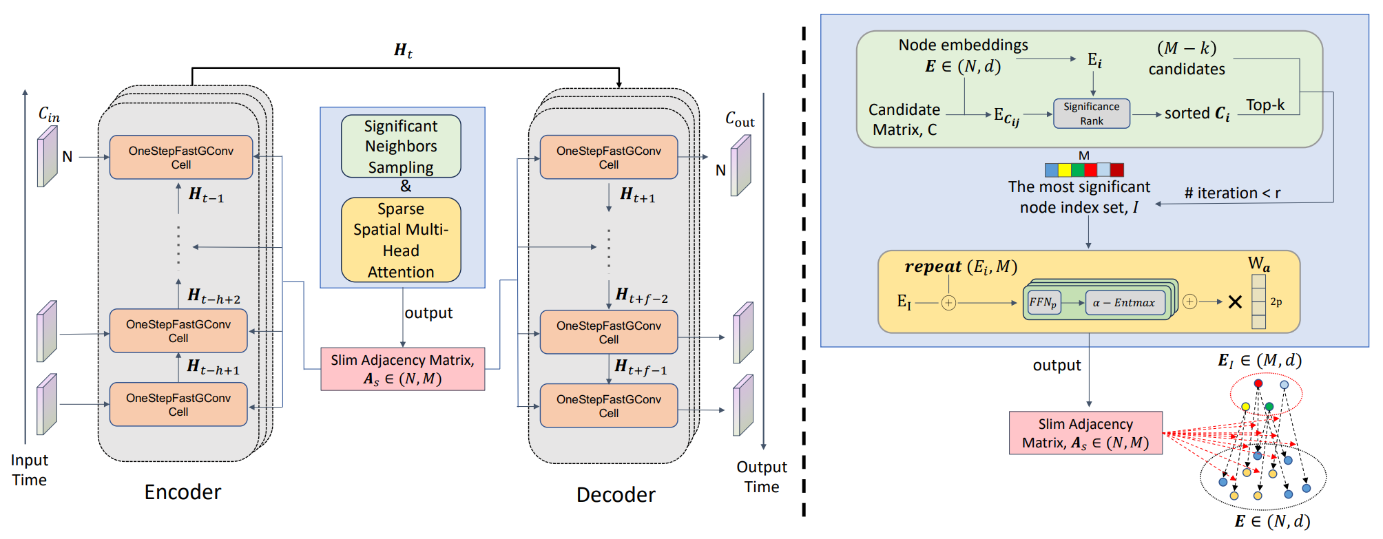
In previous articles, we have systematically examined the framework’s key building blocks. We implemented the Significant Neighbors Sampling and Sparse Spatial Multi-Head Attention modules step by step using MQL5 and OpenCL. In this process, we did not simply replicate the original algorithm verbatim — on the contrary, we implemented a number of important optimizations aimed at improving the model’s computational efficiency and stability. Thus, instead of the iterative α-Entmax function, which requires significant resources due to the search for the optimal parameter τ, we used the lighter and more stable Sparse-SoftMax. This made it possible to preserve the concept of selectively filtering out insignificant elements and reduce the load on the processor. In addition, the procedure for forming connections in the neighbor sampling module was improved. We organized a parallel evaluation of previously selected and random candidates, which allowed us to increase the diversity of connections and reduce the likelihood of losing potentially useful information.

Now that the mechanisms for constructing the graph and distributing weights among its nodes are in place, it is time to move on to the next logical step — implementing the OneStepFastGConv module. This component plays a special role in the SAGDFN architecture, as it is responsible for aggregating spatial information and generating the features on which the final forecast will be based.

Recurrent Graph Convolution Object

Continuing the line of reasoning from the previous article, where we have already assembled the graph structure (Significant Neighbors Sampling) and learned how to carefully distribute weights among key connections (Sparse Spatial Multi-Head Attention), we now turn to the heart of the recurrent block — fast graph convolution. This is not our first foray into the world of recurrent graph modules: in HimNet, we used GCRU, and it performed very well on dense structures. But in SAGDFN, the landscape is different. We deliberately work with a sparse matrix of interdependencies, and it is precisely this sparsity that dictates a different algorithmic approach. To avoid building a house on sand, let's start with the basic operation on which OneStepFastGConv will rest: efficiently multiplying a sparse matrix by a dense matrix.

This stage is crucial because it is precisely what will allow us to efficiently integrate the sparse relationship structure obtained earlier into the overall data processing context. To do this, we create a kernel in the OpenCL program that performs this operation as simply as possible while prioritizing performance and memory efficiency.

__kernel void SparseMatMult(__global const float *sparse_index,
                            __global const float *sparse_data,
                            __global const float *full,
                            __global float *result,
                            const int full_rows
                           )
  {
   const size_t sparse_row = get_global_id(0);
   const size_t sparse_col = get_local_id(1);
   const size_t full_col = get_global_id(2);
   const size_t sparse_rows = get_global_size(0);
   const size_t sparse_cols = get_local_size(1);
   const size_t full_cols = get_global_size(2);
//---
   __local float Temp[LOCAL_ARRAY_SIZE];

At the very beginning of its execution, the kernel determines the coordinates of the task being performed: the row and column indices of the sparse matrix, with the latter grouped into local groups. It also determines the column index of the dense matrix. These parameters form a kind of coordinate triplet that allows each work-item to know exactly which section of data it is responsible for. Next, the sizes of all dimensions are determined. They are necessary for correctly addressing elements.

After that, a local array Temp is allocated, which is used for synchronization and summing intermediate values within the work-group.

In the next step, each work-item determines the memory offset for the current element of the sparse matrix and retrieves the index of the corresponding row in the dense matrix.

   const int shift_sparse = RCtoFlat(sparse_row, sparse_col, sparse_rows, sparse_cols, 0);
   const int full_row = sparse_index[shift_sparse];
   const int shift_full = RCtoFlat(full_row, full_col, full_rows, full_cols, 0);

If this index is within the valid range, the product of the sparse matrix coefficient and the dense matrix element is computed. Otherwise, a zero value is used, which helps prevent incorrect operations.

   float res = (full_row >= 0 && full_row < full_rows ?
                IsNaNOrInf(sparse_data[shift_sparse] * full[shift_full], 0) : 0);
   res = LocalSum(res, 1, Temp);

The resulting partial product is passed to a local summation procedure, which accumulates the results from all work-items in the work-group. As soon as the summation is complete, the first work-item in each group (with a local column index of zero) writes the final value to the result matrix. This achieves a balance between computational parallelism and control over data writing, thereby preventing access conflicts.

   if(sparse_col == 0)
     {
      const int shift_result = RCtoFlat(sparse_row, full_col, sparse_rows, full_cols, 0);
      result[shift_result] = res;
     }
  }

This approach ensures optimal use of GPU resources. Each work-item performs only its own part of the work, and the collective summation ensures the accuracy and consistency of the final result.

After we have implemented the forward pass and learned how to carefully collect neighbors' contributions into the resulting features, the next step is the backward pass: correctly distributing the error gradient across all participating elements. The algorithm is implemented in the SparseMatMultGrad kernel, which takes the following as input:

• indices and weights of a sparse matrix,
• a buffer for gradients with respect to these weights,
• a dense matrix and its gradient buffer,
• an array of result gradients,
• the sizes of all dimensions.

These parameters define the context: we know where to look for matches between rows, which weights to use, and which accumulations to perform.

__kernel void SparseMatMultGrad(__global const float *sparse_index,
                                __global const float *sparse_data,
                                __global float *sparse_gr,
                                __global const float *full,
                                __global float *full_gr,
                                __global const float *result_gr,
                                const int sparse_rows,
                                const int sparse_cols,
                                const int full_rows,
                                const int full_cols
                               )
  {
   const size_t row_id = get_global_id(0);
   const size_t local_id = get_local_id(1);
   const size_t col_id = get_global_id(2);
   const size_t total_rows = get_global_size(0);
   const size_t total_local = get_local_size(1);
   const size_t total_cols = get_global_size(2);
//---
   __local float Temp[LOCAL_ARRAY_SIZE];

In the kernel body, each work-item receives its own coordinates in the task space:

• row_id — the row being processed in the matrix;
• local_id — the local identifier within a group;
• col_id — the matrix column.

The dimensions total_rows, total_local, and total_cols are used for convenient calculations and navigation through arrays.

The local memory buffer Temp is allocated for reductions and for transferring small portions of data between work-items within the same work-group. This is the primary coordination tool: it lets work-items exchange intermediate results and synchronize.

It should be noted here that, in this kernel, we need to distribute the error gradients between two matrices of different sizes. Both the row and column identifiers are reference points specifically in the matrix with respect to which the gradients are being computed. To that end, when queuing the kernel for execution, we plan to use the maximum values from both matrices. The excess work-items are filtered out within the kernel.

First comes the block for calculating the error gradients with respect to the weights of the sparse matrix. First, we guard the index: if the current position is within the valid range, the work-item computes shift_sparse — a flat offset in the index and data arrays of the sparse matrix.

//--- Calculate sparse gradient
   if(row_id < sparse_rows && col_id < sparse_cols)
     {
      float grad = 0;
      int shift_sparse = 0;
      if(local_id == 0)
        {
         shift_sparse = RCtoFlat(row_id, col_id, sparse_rows, sparse_cols, 0);
         Temp[0] = sparse_index[shift_sparse];
        }
      BarrierLoc;
      uint full_row = (uint)Temp[0];

The work-item whose local_id is 0 reads the corresponding index and stores it in the first element of the local memory buffer so that the other work-items can use this value without additional global accesses.

After the barrier, all work-items in the work-group know the row index of the dense matrix.

Please note: it is important to verify the correctness of the obtained row index. After the control checks pass, each work-item iterates over its assigned positions in the feature dimension and accumulates the element's contribution.

      if(full_row < (uint)full_rows)
         for(int i = local_id; i < full_cols; i += total_local)
           {
            int shift_result = RCtoFlat(row_id, i, sparse_rows, full_cols, 0);
            int shift_full = RCtoFlat(full_row, i, full_rows, full_cols, 0);
            grad += IsNaNOrInf(result_gr[shift_result] * full[shift_full], 0);
           }

This is a classic scalar accumulation over features: we take the gradient of the result with respect to each feature and multiply it by the value of the corresponding cell in the dense matrix, summing over all features.

After the local traversal is complete, a reduction is performed across the work-items in the work-group to obtain the total contribution for the given (row_id, col_id) pair.

      grad = LocalSum(grad, 1, Temp);
      if(local_id == 0)
         sparse_gr[shift_sparse] = grad;
     }

Only one work-item writes the work-group's final result to the corresponding element of the global sparse_gr buffer.

Moving on to the second major part (computing the gradient with respect to the dense matrix), we encounter the inverse problem. For each element of the dense matrix, we need to carefully sum its contribution to the block's output. However, here we encounter the problem of lacking an explicit association with the elements of the sparse matrix. Therefore, we will have to scan the entire index matrix of the sparse matrix in search of the required pointers. This is precisely the task we will assign to the work-items in the local work-group.

First, we set up a loop to iterate through the rows of the error-gradient tensor. Let me remind you that the number of rows in the error-gradient tensor and in the sparse matrix is the same.

//--- Calc full gradient
   if(row_id < full_rows && col_id < full_cols)
     {
      float grad = 0;
      for(int r = 0; r < sparse_rows; r ++)
        {
         float s = 0;
         for(int c = local_id; c < sparse_cols; c += total_local)
           {
            int shift_sparse = RCtoFlat(r, c, sparse_rows, sparse_cols, 0);
            if((int)sparse_index[shift_sparse] == (int)row_id)
              {
               s = sparse_data[shift_sparse];
               break;
              }
           }

Inside the loop, we try to find a pointer to the current row of the dense matrix among the sparse matrix indices. To ensure efficient parallelism, each work-item in the local work-group scans only a portion of the columns of the sparse matrix and, on the first match, retrieves the attention coefficient and stops the search.

Let me remind you that, during the process of selecting the nearest neighbors, we implemented a mechanism to exclude duplicates. Therefore, we do not expect connections to appear more than once in any row of the sparse matrix.

Next, we use LocalSum to aggregate the attention coefficients from all work-items in the work-group.

         s = LocalSum(s, 1, Temp);
         if(s != 0 && local_id == 0)
           {
            int shift_result = RCtoFlat(r, col_id, sparse_rows, full_cols, 0);
            grad += IsNaNOrInf(s * result_gr[shift_result], 0);
           }
        }

If the sum is nonzero, the first work-item of the work-group multiplies the resulting weight by the value of the corresponding element from the block's error gradient buffer and accumulates it in the variable grad.

After all iterations of the loop nest are completed and the total error gradient from all dependent elements has been accumulated, the first work-item of the work-group writes the accumulated value to the global buffer full_gr.

      if(local_id == 0)
        {
         int shift_full = RCtoFlat(row_id, col_id, full_rows, full_cols, 0);
         full_gr[shift_full] = grad;
        }
     }
  } 

Now that the preparatory work is complete, let's move on to the practical implementation of the OneStepFastGConv recurrent block within the main program. Here, we implement the proposed approaches within the CNeuronFastGConv class, which is designed as a compact container for all intermediate buffers and logic. The class structure is shown below.

class CNeuronFastGConv   :     public CNeuronBaseOCL
  {
protected:
   CNeuronBaseOCL          cInpAndHidden;
   CNeuronBaseOCL          cNormAttention;
   CNeuronBaseOCL          cInvDiag;
   CNeuronBaseOCL          cAX;
   CNeuronBaseOCL          cAXplusX;
   CNeuronBaseOCL          cNormAXplusX;
   CNeuronConvOCL          cZ_R;
   CNeuronBaseOCL          cZ;
   CNeuronBaseOCL          cR;
   CNeuronBaseOCL          cCandidate;
   CNeuronConvOCL          cHC;
   //---
   virtual bool      RandomWalk(CBufferFloat* data,
                                CBufferFloat* normal,
                                CBufferFloat* inv_diag,
                                const int rows,
                                const int cols
                               );
   //---
   virtual bool      feedForward(CNeuronBaseOCL *NeuronOCL) override { return false; }
   virtual bool      feedForward(CNeuronBaseOCL *NeuronOCL, CBufferFloat *SecondInput)  override { return false; };
   virtual bool      calcInputGradients(CNeuronBaseOCL *NeuronOCL) override { return false; }
   virtual bool      calcInputGradients(CNeuronBaseOCL *NeuronOCL,
                                        CBufferFloat *SecondInput,
                                        CBufferFloat *SecondGradient,
                                        ENUM_ACTIVATION SecondActivation = None
                                       ) override { return false; }
   //---
   virtual bool      updateInputWeights(CNeuronBaseOCL *NeuronOCL) override;

public:
                     CNeuronFastGConv(void) {};
                    ~CNeuronFastGConv(void) {};
   //---
   virtual bool      Init(uint numOutputs, uint myIndex, COpenCLMy *open_cl,
                          uint units, uint window, uint sparse_dimension,
                          ENUM_OPTIMIZATION optimization_type, uint batch);
   //---
   virtual bool      FeedForward(CNeuronBaseOCL *SourceData, CNeuronSNSMHAttention *SparseAttent);
   virtual bool      CalcInputGradients(CNeuronBaseOCL *SourceData, CNeuronSNSMHAttention *SparseAttent);
   //---
   virtual int       Type(void)   const   {  return defNeuronFastGConv;   }
   //--- methods for working with files
   virtual bool      Save(int const file_handle);
   virtual bool      Load(int const file_handle);
   //---
   virtual bool      WeightsUpdate(CNeuronBaseOCL *source, float tau) override;
   virtual void      SetOpenCL(COpenCLMy *obj) override;
   virtual void      SetActivationFunction(ENUM_ACTIVATION value) override { };
   //---
   virtual uint      GetCount(void) const { return (uint)cInvDiag.Neurons(); }
   virtual uint      GetSparseDimension(void) const { return (uint)cNormAttention.Neurons() / GetCount(); }
   virtual uint      GetWindow(void) const { return (uint)Neurons() / GetCount(); }
  };

In the structure of the new class, we see quite a large number of internal objects. However, they are all declared statically, which allows us to leave the class's constructor and destructor empty. The entire algorithm for configuring the object's architecture has been moved to the Init initialization method.

bool CNeuronFastGConv::Init(uint numOutputs, uint myIndex, COpenCLMy *open_cl,
                            uint units, uint window, uint sparse_dimension,
                            ENUM_OPTIMIZATION optimization_type, uint batch)
  {
   if(!CNeuronBaseOCL::Init(numOutputs, myIndex, open_cl, units * window, optimization_type, batch))
      return false;
   activation = None;

The first line inside the method passes control to the parent class. This involves the basic binding of the layer to the OpenCL context and the creation of all the inherited interfaces required for the module to function within the model. If this initialization fails, there is no point in continuing the method, so we immediately return false. This early exit protects against further errors and unnecessary allocations.

Immediately after that, we explicitly disable the activation function. This makes sense: the block itself controls the activations in its components (sigmoids for gates, tanh for candidates), so there is no need for an external global activation here.

Next comes the process of initializing the internal components. The first object is designed to concatenate the previous hidden state and the input data.

   int index = 0;
   if(!cInpAndHidden.Init(0, index, OpenCL, 2 * units * window, optimization, iBatch))
      return false;

The next line creates cNormAttention. This is where the slim attention matrix As is stored after normalization. It will receive weights from the Sparse Attention module.

   index++;
   if(!cNormAttention.Init(0, index, OpenCL, units * sparse_dimension, optimization, iBatch))
      return false;
   index++;
   if(!cInvDiag.Init(0, index, OpenCL, units, optimization, iBatch))
      return false;

Let's move on to cInvDiag — a vector of inverses of the diagonal entries that will be used to multiply the rows of the diffusion result during normalization.

Next, cAX is created. This buffer stores the result of SpMM. Its size is based on cInpAndHidden, which ensures dimensional compatibility with the subsequent steps.

   index++;
   if(!cAX.Init(0, index, OpenCL, cInpAndHidden.Neurons(), optimization, iBatch))
      return false;
   index++;
   if(!cAXplusX.Init(0, index, OpenCL, cInpAndHidden.Neurons(), optimization, iBatch))
      return false;
   index++;
   if(!cNormAXplusX.Init(0, index, OpenCL, cInpAndHidden.Neurons(), optimization, iBatch))
      return false;

After cAX comes cAXplusX — a buffer for the sum AX + X. Here, we explicitly store the intermediate result before applying the diagonal inversion. Such an explicit buffer makes debugging easier and provides control over the order of operations.

Next, cNormAXplusX is created — the final normalized tensor (D+I)^-1(AX + X). It is then fed into a GRU-like block. If it is missing, the update-gate mechanics break, so once again this check is critical.

Next, cZ_R is initialized. This is a compact convolutional layer that will simultaneously generate logits for the Z and R gates. Here, we use the sigmoid function as the activation function. This approach is simple and reliable: the gates are always within the range [0,1].

   index++;
   if(!cZ_R.Init(0, index, OpenCL, 2 * window, 2 * window, 2 * window, units, 1, optimization, iBatch))
      return false;
   cZ_R.SetActivationFunction(SIGMOID);
   index++;
   if(!cZ.Init(0, index, OpenCL, window * units, optimization, iBatch))
      return false;
   index++;
   if(!cR.Init(0, index, OpenCL, window * units, optimization, iBatch))
      return false;

The next two buffers, cZ and cR, are created to separate the gate values. Having separate buffers simplifies the step-by-step logic for updating the hidden state.

Initializing cCandidate creates a buffer for the intermediate concatenated input to the candidate block.

   index++;
   if(!cCandidate.Init(0, index, OpenCL, 2 * window * units, optimization, iBatch))
      return false;
   index++;
   if(!cHC.Init(0, index, OpenCL, 2 * window, 2 * window, window, units, 1, optimization, iBatch))
      return false;
   cHC.SetActivationFunction(TANH);
//---
   return true;
  }

The cHC block is the actual computation of the Candidate Hidden State. Using TANH as the activation function is standard practice that keeps the candidate values bounded and stable in scale.

Once all the calls within the Init method have completed successfully, we return true at the very end, indicating that the layer is configured and ready to run.

Let's move smoothly from initialization to execution. Now that everything is allocated and configured, the FeedForward method is a live data flow through OneStepFastGConv.

bool CNeuronFastGConv::FeedForward(CNeuronBaseOCL *SourceData, CNeuronSNSMHAttention *SparseAttent)
  {
   if(!SourceData || !SparseAttent)
      return false;
//---
   const uint units = GetCount();
   const uint window = GetWindow();
   const uint sparse = GetSparseDimension();

First, the method checks the inputs to ensure that the pointers to the source data objects are valid. This is a simple but essential safeguard: if there is no data source or sparse attention module, execution cannot continue. This early exit prevents uncontrolled failures and provides predictable diagnostics.

Next, we retrieve the layer's configuration parameters. It is very convenient to keep these variables local: reading them through class methods in a hot loop is slower and less clear.

The following line launches RandomWalk. This is a preprocessing step for the attention matrix. RandomWalk collects statistics across the rows of the slim matrix and performs smooth normalization. It then writes cNormAttention (N×M) and cInvDiag (N), the inverse diagonal values for subsequent normalization. It is important to note that RandomWalk runs in parallel on the GPU, carefully summing over M and returning stable inv_diag values. If this step fails, it is better to interrupt execution: all subsequent normalizations depend on it.

   if(!RandomWalk(SparseAttent.getOutput(), cNormAttention.getOutput(), cInvDiag.getOutput(), window, sparse))
      return false;
   if(!SwapOutputs())
      return false;
   if(!Concat(SourceData.getOutput(), PrevOutput, cInpAndHidden.getOutput(), window, window, units))
      return false;

After that, SwapOutputs is executed. This is an internal mechanism of the layer that swaps the pointers to the previous and current outputs (rolling buffer). The swap ensures that PrevOutput contains Ht-1, while the current Output is free for writing.

Next, the input for SpMM/GRU is assembled. Here, concatenation is performed along the channel dimension: for each row, a vector is formed that combines the current observed fragment Xt and the previous hidden state Ht-1.

Once the preparatory work is complete, the key operation is performed: multiplying the sparse attention matrix by the previously prepared dense matrix of concatenated input data and the hidden state.

   if(!SparseMatMul(SparseAttent.GetIndexes(), cNormAttention.getOutput(), cInpAndHidden.getOutput(),
                                                  cAX.getOutput(), units, sparse, units, 2 * window))
      return false;
   if(!SumAndNormilize(cAX.getOutput(), cInpAndHidden.getOutput(), cAXplusX.getOutput(),
                                                         2 * window, false, 0, 0, 0, 1))
      return false;

Next, the sum with Self-Loop is performed. Here we add AX+X.

The next step is to apply diagonal normalization.

   if(!DiagMatMul(cInvDiag.getOutput(), cAXplusX.getOutput(), cNormAXplusX.getOutput(), units, 2 * window, 1, None))
      return false;

This is simple channel-wise multiplication of the rows by the precomputed inv_diag.

Next, the logits for the gates are calculated. The cZ_R convolutional layer receives normalized aggregated features and returns a 2×hidden vector (logits for Z and R). Since the SIGMOID activation function was set during the initialization phase, this operation results in values in the range [0,1].

   if(!cZ_R.FeedForward(cNormAXplusX.AsObject()))
      return false;
   if(!DeConcat(cZ.getOutput(), cR.getOutput(), cZ_R.getOutput(), window, window, units))
      return false;

Next, we split the resulting logits into separate buffers.

This is immediately followed by element-wise multiplication of the Reset gate by the previous hidden state. This forms R⊙Ht-1. The result is then used as a modified version of the hidden state to generate candidates.

   if(!ElementMult(cR.getOutput(), PrevOutput, cR.getPrevOutput()))
      return false;

Next, the candidate input is formed: we concatenate R⊙Ht-1 with the current Xt.

   if(!Concat(SourceData.getOutput(), cR.getPrevOutput(), cCandidate.getOutput(), window, window, units))
      return false;
   if(!cHC.FeedForward(cCandidate.AsObject()))
      return false;
   if(!GateElementMult(PrevOutput, cHC.getOutput(), cZ.getOutput(), Output))
      return false;
//---
   return true;
  }

Calling the forward pass method of the cHC convolutional layer performs a nonlinear transformation and applies tanh, returning a candidate hidden state. The final composition then forms the new hidden state.

From the description of the forward pass, we move on to the backward chain — now we need to carefully examine how the error flows backward through all the links of OneStepFastGConv. The process is implemented in the CalcInputGradients method.

bool CNeuronFastGConv::CalcInputGradients(CNeuronBaseOCL *SourceData, CNeuronSNSMHAttention *SparseAttent)
  {
   if(!SourceData || !SparseAttent)
      return false;
//---
   const uint units = GetCount();
   const uint window = GetWindow();
   const uint sparse = GetSparseDimension();

The method immediately safeguards itself: if there are no valid pointers to the source data objects, there is nothing to execute. We then correctly terminate the operation with a result of false. This is a simple but necessary check—it is better to interrupt the training pass early than to end up with mysterious NaN values later.

Next, the configuration parameters are retrieved. These numbers define the shape of all gradient tensors and are needed for correct addressing.

The first actual call is GateElementMultGrad. This is the reverse of the final composition Ht = Z⊙Ht-1+(1−Z)⊙H̃.

   if(!GateElementMultGrad(PrevOutput, cInpAndHidden.getGradient(),
                           cHC.getOutput(), cHC.getGradient(),
                           cZ.getOutput(), cZ.getGradient(),
                           Gradient, None, cHC.Activation(), cZ_R.Activation()))
      return false;

The function computes three things simultaneously: the gradient with respect to H̃ (candidates), with respect to Z (update gate), and with respect to Ht-1 (the previous hidden state), carefully decomposing the total gradient into its components.

Next, we propagate the error gradient through the candidate-generation convolutional layer.

   if(!cCandidate.CalcHiddenGradients(cHC.AsObject()))
      return false;
   if(!DeConcat(SourceData.getGradient(), cR.getPrevOutput(),
                cCandidate.getGradient(), window, window, units))
      return false;

Next, we will split the resulting gradients into two parts — the influence of the input data and R⊙Ht-1.

Then ElementMultGrad distributes the contributions of the reset gate and the previous hidden state.

   if(!ElementMultGrad(cR.getOutput(), cR.getGradient(),
                       PrevOutput, cInpAndHidden.getGradient(),
                       cR.getPrevOutput(), cZ_R.Activation(), None))
      return false;

The next step is to combine the local gradients with respect to Z and R back into a flat vector of logits, which we feed into cZ_R for the layer's backpropagation.

   if(!Concat(cZ.getGradient(), cR.getGradient(),
              cZ_R.getGradient(), window, window, units))
      return false;
   if(!cNormAXplusX.CalcHiddenGradients(cZ_R.AsObject()))
      return false;
   if(!DiagMatMulGrad(cInvDiag.getOutput(), cInvDiag.getGradient(),
                      cAXplusX.getOutput(), cAX.getGradient(),
                      cNormAXplusX.getGradient(), units, 2 * window, 1))
      return false;
   if(!SparseMatMulGrad(SparseAttent.GetIndexes(), cNormAttention.getOutput(),
                        cNormAttention.getGradient(), cInpAndHidden.getOutput(),
                        cInpAndHidden.getGradient(), cAX.getGradient(),
                        units, sparse, units, 2 * window))
      return false;

Next, we run the backward pass through the convolutional layer that generates the gate logits. As a result, we obtain the gradient with respect to cNormAXplusX — that is, with respect to the normalized aggregated input.

This is followed by a series of iterations in which the error gradients are distributed between the concatenated input-data tensor and the normalized attention coefficients. First, we backpropagate the gradient through the diagonal normalization. Then we unroll SpMM and distribute the gradients to the normalized attention weights and the concatenated features.

It is important to note that after executing SparseMatMulGrad, we need to sum the error gradient of the concatenated feature tensor from the two data paths.

   if(!SumAndNormilize(cAX.getGradient(), cInpAndHidden.getGradient(),
                      cInpAndHidden.getGradient(), 2 * window, false, 0, 0, 0, 1))
      return false;

Next, we need to collect the error gradients at the input-data level. Here we need to remember that we used the input data in two data paths: the primary feature concatenation and the tensor concatenation for the candidates. We have already propagated the error gradient from the second data path. Now we need to extract the values from the second data path and add them to the values obtained earlier.

   if(!DeConcat(cAXplusX.getGradient(), cAXplusX.getPrevOutput(),
                cInpAndHidden.getGradient(), window, window, units))
      return false;
   if(!SumAndNormilize(SourceData.getGradient(), cAXplusX.getGradient(),
                      SourceData.getGradient(), window, false, 0, 0, 0, 1))
      return false;
   if(SourceData.Activation() != None)
      if(!DeActivation(SourceData.getOutput(), SourceData.getGradient(),
                       SourceData.getGradient(), SourceData.Activation()))
         return false;

It is also necessary to check for an activation function on the input-data tensor. If necessary, we adjust the obtained values by its derivative.

The final significant step is to transfer the error gradient from the normalized attention matrix cNormAttention to its original state SparseAttent. In the forward pass, we performed normalization, and now we pass the gradients back through this diagonal step into the form expected by the SparseAttent module.

   if(!DiagMatMul(cInvDiag.getOutput(), cNormAttention.getGradient(),
                  SparseAttent.getGradient(), units, sparse, 1, None))
      return false;
//---
   return true;
  }

At the end, the method returns true, which means that all gradients have correctly propagated backward and been accurately accumulated for the corresponding inputs and internal parameters.

This concludes our discussion of the algorithms used to implement the methods of the CNeuronFastGConv class. The complete code for this object and all of its methods is provided in the attachment.

Top-Level SAGDFN Object

After constructing the object of a single recurrent block, we move on to the top level — the wrapper that connects the Encoder and Decoder into a unified system. The CNeuronSAGDFN class is more than just a container: it organizes the data flow, manages the sharing of the same slim adjacency matrix, and ensures the consistency of temporal and spatial transformations throughout the model.

class CNeuronSAGDFN  :  public CNeuronTransposeOCL
  {
protected:
   CNeuronTransposeOCL     cTranspose;
   CLayer                  cEmbedding;
   CNeuronSNSMHAttention   cAttention;
   CLayer                  cGCRU;
   CLayer                  cProjection;
   //---
   virtual bool      feedForward(CNeuronBaseOCL *NeuronOCL) override;
   virtual bool      calcInputGradients(CNeuronBaseOCL *NeuronOCL) override;
   virtual bool      updateInputWeights(CNeuronBaseOCL *NeuronOCL) override;

public:
                     CNeuronSAGDFN(void) {};
                    ~CNeuronSAGDFN(void) {};
   //---
   virtual bool      Init(uint numOutputs, uint myIndex, COpenCLMy *open_cl,
                          uint time_steps, uint variables, uint embedding_dim,
                          uint emb_layers, uint sparse_dimension, uint heads,
                          float sparse, uint gcru_layers,
                          uint forecast, uint forec_layers,
                          ENUM_OPTIMIZATION optimization_type, uint batch);
   //---
   virtual int       Type(void)   const   {  return defNeuronSAGDFN;   }
   //--- methods for working with files
   virtual bool      Save(int const file_handle);
   virtual bool      Load(int const file_handle);
   //---
   virtual bool      WeightsUpdate(CNeuronBaseOCL *source, float tau) override;
   virtual void      SetOpenCL(COpenCLMy *obj) override;
   virtual void      SetActivationFunction(ENUM_ACTIVATION value) override {};
  };

When organizing the operation of the CNeuronSAGDFN class, it is important to note that the SAGDFN framework is built on identifying key spatial dependencies by analyzing correlations between univariate sequences in a multimodal time series. We, on the other hand, usually work with time series. Therefore, within the object, we implemented transposition of the source data tensor and inverse transposition of the result tensor.

To perform the first operation, we declare the corresponding internal object, while the latter is planned to be performed by means of the parent class, CNeuronTransposeOCL. This solution simplifies the task of preparing data before feeding it into the module and makes it easier to integrate the model into the existing pipeline.

In addition, we have provided the ability to dynamically change the object's architecture. To do this, three dynamic arrays were included:

• cEmbedding — a mini-model for generating embeddings of a specified size from the input data;
• cGCRU — a stack of sequential GCRU (Graph-Convolutional Recurrent Unit) units that aggregates a sequence of OneStepFastGConv blocks;
• cProjection — a projection block that converts hidden representations into target predictions in the decoder.

This approach makes it possible to flexibly increase the depth of the recurrent stack and experiment with the number of diffusion steps. CNeuronSAGDFN combines input transposition, embedding, shared Attention, and a GCRU stack into a single Encoder-Decoder. It manages how the same slim adjacency matrix is reused throughout the stack, ensures data format compatibility, and serves as the central orchestrator during training.

The actual construction of the new object's architecture takes place in the Init method.

bool CNeuronSAGDFN::Init(uint numOutputs, uint myIndex, COpenCLMy *open_cl,
                         uint time_steps, uint variables, uint embedding_dim,
                         uint emb_layers, uint sparse_dimension, uint heads,
                         float sparse, uint gcru_layers,
                         uint forecast, uint forec_layers,
                         ENUM_OPTIMIZATION optimization_type, uint batch)
  {
   if(emb_layers <= 0 || gcru_layers <= 0 || forec_layers <= 0)
      return false;

In the body of the method, simple validation of the received parameters is performed first — if the number of layers in any of the blocks is zero, initialization is immediately terminated. This is an honest and useful check: it is better to reject the input data than to continue building an incorrect structure.

Control is then passed to the method of the same name in the parent class, which defines the neuron's general structure and reserves the basic resources. If this step fails, we likewise cleanly return false, because everything that follows depends on a correct base context.

   if(!CNeuronTransposeOCL::Init(numOutputs, myIndex, open_cl, variables, forecast, optimization_type, batch))
      return false;

Next, we initialize an object to transpose the source data tensor into the expected format.

   uint index = 0;
   if(!cTranspose.Init(0, index, OpenCL, time_steps, variables, optimization, iBatch))
      return false;

Next, we begin assembling the embedding mini-model. We clear the container and bind the OpenCL context. The first convolutional block adjusts the data dimensionality to the specified level. We add it to the cEmbedding container and assign SoftPlus as its activation function.

//--- Embedding
   cEmbedding.Clear();
   cEmbedding.SetOpenCL(OpenCL);
   index++;
   CNeuronConvOCL *conv = new CNeuronConvOCL();
   if(!conv ||
      !conv.Init(0, index, OpenCL, time_steps, time_steps, embedding_dim, variables, 1, optimization, iBatch) ||
      !cEmbedding.Add(conv))
     {
      DeleteObj(conv);
      return false;
     }
   conv.SetActivationFunction(SoftPlus);
   for(uint i = 1; i < emb_layers; i++)
     {
      index++;
      conv = new CNeuronConvOCL();
      if(!conv ||
         !conv.Init(0, index, OpenCL, embedding_dim, embedding_dim,
                    embedding_dim, variables, 1, optimization, iBatch) ||
         !cEmbedding.Add(conv))
        {
         DeleteObj(conv);
         return false;
        }
      conv.SetActivationFunction(SoftPlus);
     }

Next, in the loop over emb_layers, we add additional convolutional layers with the SoftPlus activation function. This results in a deep embedding stack with the same channel width.

After the convolutions, we add BatchNorm — a separate object that normalizes the output of the last convolutional layer.

   CNeuronBatchNormOCL *norm = new CNeuronBatchNormOCL();
   index++;
   if(!norm ||
      !norm.Init(0, index, OpenCL, conv.Neurons(), iBatch, optimization) ||
      !cEmbedding.Add(norm))
     {
      DeleteObj(norm);
      return false;
     }
   norm.SetActivationFunction(None);

Next, we prepare the GCRU blocks. We clear the cGCRU container, bind OpenCL, and immediately initialize cAttention.

//--- GCRUs
   cGCRU.Clear();
   cGCRU.SetOpenCL(OpenCL);
   index++;
   if(!cAttention.Init(0, index, OpenCL, variables, embedding_dim, heads,
                       sparse_dimension, sparse, optimization, iBatch))
      return false;

Note that cAttention is initialized before the gcru objects are created — this is intentional and correct, because all GCRU blocks will read the same slim adjacency matrix. If attention initialization fails, we stop and signal the error.

Next, in a loop, we create the required number of CNeuronFastGConv objects. If any gcru fails to be created, we delete it and return false. This forms a stack of recurrent graph blocks, all of which will jointly operate on the matrix created by cAttention.

   CNeuronFastGConv *gcru = NULL;
   for(uint i = 0; i < gcru_layers; i++)
     {
      index++;
      gcru = new CNeuronFastGConv();
      if(!gcru ||
         !gcru.Init(0, index, OpenCL, variables, embedding_dim, sparse_dimension, optimization, iBatch) ||
         !cGCRU.Add(gcru))
        {
         DeleteObj(gcru);
         return false;
        }
     }

After that, the projection block cProjection is constructed. The first convolutional layer transforms the data from the embedding dimension into the forecast space for each variable.

//--- Forecast
   cProjection.Clear();
   cProjection.SetOpenCL(OpenCL);
   index++;
   conv = new CNeuronConvOCL();
   if(!conv ||
      !conv.Init(0, index, OpenCL, embedding_dim, embedding_dim,
                 forecast, variables, 1, optimization, iBatch) ||
      !cProjection.Add(conv))
     {
      DeleteObj(conv);
      return false;
     }
   conv.SetActivationFunction(SoftPlus);
   for(uint i = 1; i < forec_layers; i++)
     {
      index++;
      conv = new CNeuronConvOCL();
      if(!conv ||
         !conv.Init(0, index, OpenCL, forecast, forecast,
                    forecast, variables, 1, optimization, iBatch) ||
         !cProjection.Add(conv))
        {
         DeleteObj(conv);
         return false;
        }
      conv.SetActivationFunction(SoftPlus);
     }
   norm = new CNeuronBatchNormOCL();
   index++;
   if(!norm ||
      !norm.Init(0, index, OpenCL, conv.Neurons(), iBatch, optimization) ||
      !cProjection.Add(norm))
     {
      DeleteObj(norm);
      return false;
     }
   norm.SetActivationFunction(None);
//---
   return true;
  }

Next, we add additional convolutional layers in a loop. At the end of the mini-model, we add a BatchNorm layer without an external activation, just as we did in the embedding stack. If all additions were successful, Init returns true, and the architecture is built.

Moving smoothly from the structure of the layers to their execution, let’s walk through the feedForward method and see exactly what happens at runtime — which buffers move, which checks prevent crashes, and where the subtle pitfalls lie.

bool CNeuronSAGDFN::feedForward(CNeuronBaseOCL *NeuronOCL)
  {
   if(!cTranspose.FeedForward(NeuronOCL))
      return false;

The method begins by transposing the input data. This is the point where we move from a multimodal time-series representation to a set of univariate sequences. If the operation fails, continuing down the pipeline is pointless — we exit gracefully.

After that, we create local pointer variables for the internal objects. A simple but key operation that lets us reuse the same block of code with different objects.

   CNeuronBaseOCL *inputs = cTranspose.AsObject();
   CNeuronBaseOCL *current = NULL;

First, the embedding is performed. We iterate over all components of the cEmbedding container in a loop. At each iteration, we get the next layer in the current variable and immediately call its forward pass method safely. This means that each embedding layer sequentially transforms the input data and passes the result to the next one.

//--- Embedding
   for(int i = 0; i < cEmbedding.Total(); i++)
     {
      current = cEmbedding[i];
      if(!current ||
         !current.FeedForward(inputs))
         return false;
      inputs = current;
     }

After successful execution, we change the pointer in the inputs variable — that is, we shift the role of the input data to the result we have just obtained. Then we move on to the next iteration of the loop.

As a result, after all iterations of the loop have been completed, the pointer in the inputs variable points to the last embedding layer — the resulting dense representation of the time window being analyzed.

The next stage is the GCRU stack. First, we form the slim matrix As (indices and weights) based on the current representations. If the attention mechanism did not work, it is better to stop and not try further.

//--- GCRUs
   if(!cAttention.FeedForward(inputs))
      return false;
   CNeuronFastGConv *gcru = NULL;
   for(int i = 0; i < cGCRU.Total(); i++)
     {
      gcru = cGCRU[i];
      if(!gcru ||
         !gcru.FeedForward(inputs, cAttention.AsObject()))
         return false;
      inputs = gcru;
     }

Then, in a loop over the cGCRU container, we take each element in turn and call its forward pass method.

Please note: in this case, two arguments are passed — the current tensor and a reference to the attention object, from which GCRU will retrieve the indices and weights As. After each successful step, we update the pointer in the local source-data variable and move on to the next iteration.

As a result, the GCRU stack operates sequentially: each block reads the same slim matrix, but applies it to its own state and returns an updated hidden representation.

Once the stack of recurrent blocks has completed, we move on to the forecast projection block. The loop over the cProjection container follows the same logic: we take the next projection layer and call the forward pass method, then update the pointer to the source data object.

//--- Forecast
   for(int i = 0; i < cProjection.Total(); i++)
     {
      current = cProjection[i];
      if(!current ||
         !current.FeedForward(inputs))
         return false;
      inputs = current;
     }
//--- result
   return CNeuronTransposeOCL::feedforward(inputs);
  }

Conceptually, this is the transformation of the hidden representation into the final forecast shape for each variable.

Finally, we convert the data back to its original format using the parent class methods. This is a reverse transposition: the forecasts are now returned to the format expected by the rest of the system. If the last step is successful, the method will return true, and the entire forward pass chain will complete correctly.

The feedForward method is implemented in a linear and transparent manner: the data undergoes transposition, then passes through the embedding stack, receives a shared slim attention matrix, is processed sequentially by GCRU blocks, is projected into the forecast, and is returned to its original format. This data path is easy to debug and extend — you just need to take care with pointers and keep intermediate transformations efficient.

The backward pass methods are structured similarly. Therefore, I suggest not dwelling on their detailed examination. The complete code for the CNeuronSAGDFN class and all of its methods is provided in the attachment and is available for independent study.

Testing

Training the model is like a well-planned expedition: before setting out into the open seas of the real market, we practiced thoroughly in the calm harbor of history. This first, offline phase was based on data for the EURUSD currency pair on the H1 timeframe throughout 2024 — a period rich in contrasts. Here we found everything from the calm, almost mirror-like waters of sideways ranges to the turbulent storms of sharp trend moves and unexpected bursts of news-driven volatility. This wide variety of market scenarios enabled the model to develop robust navigation and learn to recognize both common and rare price movement patterns, without losing its bearings even under challenging conditions.

Once these preparations were complete, it was time to leave the training dock and put the ship to the test in the currents of the real market. The second stage — online fine-tuning — was conducted under live-fire conditions in the MetaTrader 5 Strategy Tester. Here, data arrived sequentially, one candle after another, and the model learned not only to analyze streaming data but also to maintain stability amid whirlpools of noise, on the shifting shoals of low liquidity, and during unexpected news squalls. This stage served as precision fine-tuning: it did not disrupt the framework that had already been established, but helped refine it to fit reality, thereby increasing adaptability and reducing the risk of overfitting.

The final test turned out to be a real trial by fire. We took the data for January 2025 — completely new data, untouched by previous experiments — and loaded all the previously derived parameters without making a single change. This was a crucial point: no fine-tuning, no additional adjustments — just a pure test that reflected the model's true ability to generalize.

The test results are shown below.

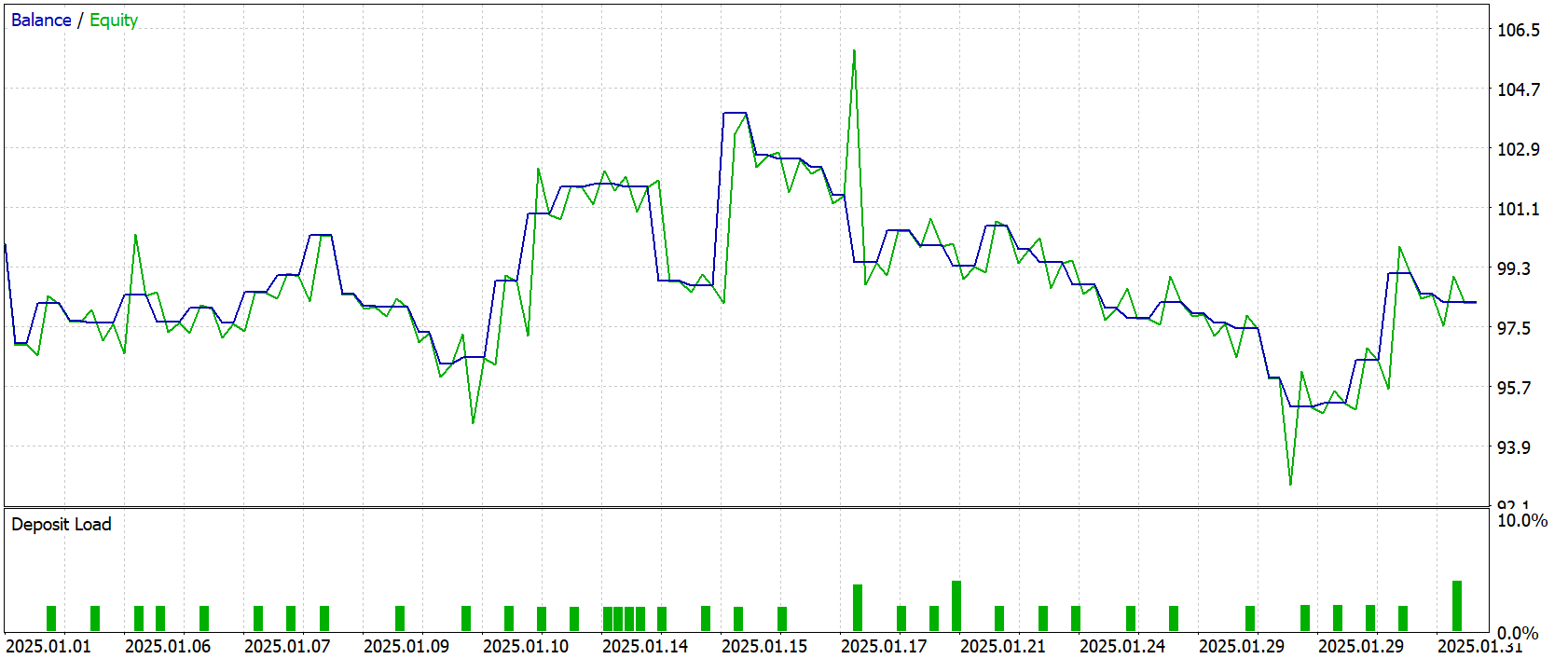
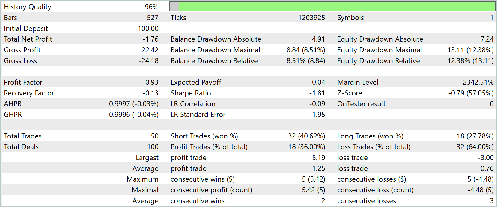
The test results showed that the model behaved cautiously and remained reasonably predictable. However, the final return was negative: -1.76 USD on an initial deposit of 100.0 USD. Gross profit amounted to 22.42 USD, but the gross losses exceeded that amount, reaching 24.18 USD. This was also reflected in the key metrics: the profit factor settled at 0.93, indicating a slight predominance of losing trades. The recovery factor also fell into negative territory, reaching -0.13.

The trade distribution shows that the model opened 50 orders, of which 32 accounted for short positions with a success rate of about 40%, while there were only 18 long trades, with a success rate of just under 28%. There were 18 profitable trades, accounting for 36% of the total, while 32 trades resulted in a loss. The longest winning streak was relatively modest — five consecutive trades that yielded a profit of about 5.42 USD — while the longest losing streak also consisted of five trades, resulting in a -4.48 USD drawdown.

The balance and equity chart shows that the strategy followed an undulating pattern, with periods of moderate growth followed by declines, without any sharp drops but also without a sustained upward trend. After the initial adaptation, a short-term uptick was observed; however, it was not sustained, and the balance gradually drifted into negative territory, fluctuating around the starting level until the end of the test period. This suggests that the algorithm has not yet established a consistent advantage over the time period in question, but it has also not experienced any catastrophic failures — the drawdown remained within 8.5% on balance and around 12% on equity.

Overall, the test results can be described as interim and as an indication that the model requires further fine-tuning and, possibly, an expanded training dataset to improve its generalization ability. It is not prone to sharp drawdowns, but it has not yet demonstrated consistent profits, which makes its behavior more conservative and cautious than risky.

Conclusion

In conclusion, we can state that the testing conducted allowed us to objectively assess the current state of the developed approach and identify its strengths and weaknesses. The model demonstrated resilience to sharp market fluctuations and a moderate level of drawdown, maintaining risk control even under adverse scenarios. However, the overall return remains negative for now, and the ratio of profitable to unprofitable trades indicates the need for further parameter optimization and, likely, an expansion of the training dataset.

These results are not a failure — on the contrary, they define the limits of the current implementation and set the direction for future development. The next steps should focus on refining the decision-making process, improving noise filtering, and enhancing forecasting accuracy in a volatile market. Thus, the framework presented here already provides a stable, functional foundation, but its potential has only been partially realized, leaving room for further improvements and practical adaptation to real-world trading tasks.

References

• SAGDFN: A Scalable Adaptive Graph Diffusion Forecasting Network for Multivariate Time Series Forecasting
• Other articles in this series

Programs used in this article

#	Name	Type	Description
1	Study.mq5	Expert Advisor	Expert Advisor for offline model training
2	StudyOnline.mq5	Expert Advisor	Expert Advisor for online model training
3	Test.mq5	Expert Advisor	Expert Advisor for model testing
4	Trajectory.mqh	Class Library	Structure for describing the system state and model architecture
5	NeuroNet.mqh	Class Library	Class library for building a neural network
6	NeuroNet.cl	Library	Code library for the OpenCL program