Neural Networks in Trading: Probabilistic Time Series Forecasting (Conclusion)

Introduction

Financial time series remain one of the most challenging types of data to analyze. Their behavior can hardly be called stable: there are no clear patterns here, but rather a combination of trends, cycles, noise, and unexpected structural shifts. For this reason, traditional models such as linear regression or moving averages, despite their simplicity and speed, prove insufficient in most cases. On the other hand, modern neural network solutions, which possess tremendous expressive power, often suffer from overfitting, instability, and a lack of interpretability.

In such circumstances, hybrid approaches that combine time-tested mathematical constructs with the flexibility of neural networks are particularly interesting. It is precisely on this balance that the K²VAE framework is built — a system designed to analyze and forecast time series while taking their real-world characteristics into account. A key advantage of this framework is its ability to capture the underlying dynamics of the system by learning from sequences of market states and adjusting its inferences as new data arrive.

The framework is based on three fundamental ideas, each of which complements the others and compensates for their weaknesses. The first is the Koopman representation, which aims to map the behavior of a nonlinear system onto a linear subspace. This transformation, albeit approximate, provides a powerful tool for description and forecasting, allowing us to work with time series not at the level of superficial statistics, but through the reconstruction of underlying dynamics.

The second idea is the use of the Kalman filter, not in its canonical form, but in a stabilized form suitable for use in stochastic neural network architectures. The Kalman filter acts as an adaptive corrector here: it refines the estimates obtained from the KoopmanNet module based on new observations, while also providing information about the level of confidence in each forecast. This is particularly valuable when the focus is not simply on forecasting prices, but on assessing the probability of certain scenarios.

The third idea is the integration of a variational autoencoder. It allows us to produce probabilistic forecasts rather than point forecasts: instead of a single possible scenario, we obtain an entire distribution that reflects both the main trend and possible deviations.

Thus, K²VAE becomes more than just another model in the analytical toolkit; it is a system capable of quantitatively describing uncertainty, taking alternative scenarios into account, and adapting to new market conditions.

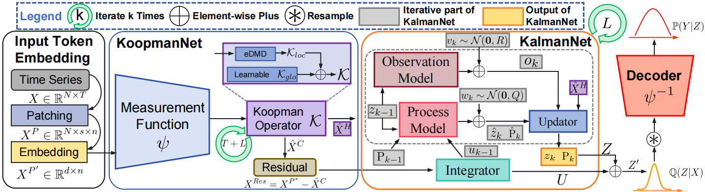
In previous articles, we have already examined the key components of this framework in detail. We described how KoopmanNet works, how the latent representation is formed, how the Kalman filter is integrated into the architecture, and how all elements are trained jointly. Particular attention was paid to computational stability and the mechanics of information propagation within the model.

Model Architecture

After the step-by-step construction of the individual components that form the architectural foundation of the K²VAE framework, we move on to the next logical stage — integrating all the elements into a single functional system.

It should be emphasized that, as in our previous work, our goal is not to construct a predictive model in its classical, isolated form. The forecast here is only a byproduct, secondary to the more fundamental task of creating an expressive and stable latent representation of the current environment state. This representation not only summarizes the incoming information but also serves as a key input for the trainable Agent when making trading decisions.

Thus, we view the K²VAE framework not as a standalone forecasting model, but as an advanced Encoder for the environment state, integrated into the previously implemented architecture based on the Actor–Director–Critic approach. Here, the VAE component serves as a mechanism for generating a probabilistic description of future scenarios, KoopmanNet is responsible for linear dynamics in the latent space, and the Kalman filter performs correction and refinement based on incoming observations. All of this serves a single purpose — to provide the Agent with a representation of the external environment that contains as much useful information as possible for making well-considered, statistically sound trading decisions.

Integrating K²VAE components into the Actor–Director–Critic architecture provides the system with the necessary depth and stability. As a result, the latent state formed by the Encoder contains information not only about the current state of affairs but also about the likely trajectories of its evolution. This qualitatively improves the behavior of the Agent: it does not simply react to current signals, but acts with possible scenarios in mind, which is particularly important in highly volatile and unpredictable market conditions.

This is where the CreateDescriptions method comes into play. It is responsible for assembling all architectural descriptions — from the Encoder and forecasting modules to the decision-making components. This method lays the foundation for future training by determining which layers will be used within each component of our system and in what order.

bool CreateDescriptions(CArrayObj *&encoder,
                        CArrayObj *&forecast1,
                        CArrayObj *&forecast2,
                        CArrayObj *&forecast3,
                        CArrayObj *&actor,
                        CArrayObj *&director,
                        CArrayObj *&critic
                       )
  {
//---
   CLayerDescription *descr;
//---
   if(!encoder)
     {
      encoder = new CArrayObj();
      if(!encoder)
         return false;
     }
   if(!forecast1)
     {
      forecast1 = new CArrayObj();
      if(!forecast1)
         return false;
     }
   if(!forecast2)
     {
      forecast2 = new CArrayObj();
      if(!forecast2)
         return false;
     }
   if(!forecast3)
     {
      forecast3 = new CArrayObj();
      if(!forecast3)
         return false;
     }
   if(!actor)
     {
      actor = new CArrayObj();
      if(!actor)
         return false;
     }
   if(!director)
     {
      director = new CArrayObj();
      if(!director)
         return false;
     }
   if(!critic)
     {
      critic = new CArrayObj();
      if(!critic)
         return false;
     }

In the method parameters, we receive pointers to a number of dynamic arrays — one for each model. These are containers that will hold the architectural descriptions of the neural network blocks. Before filling them in, we perform a mandatory check to verify that the received pointers are correct. If the required object is missing, we do not attempt to work with dangling memory; instead, we carefully create a new array instance. This step may seem like a technical formality, but in practice it is precisely what lays the foundation for the stability of all subsequent work.

After that, the main part begins — filling each array with the appropriate layers and connections that form the complete configuration of the neural network. Let's start with the central component of the system — the environment state Encoder. It is into this component that we integrate the core ideas underlying the K²VAE framework. As a reminder, the task of the Encoder is not simply to gather information about market conditions, but to create an expressive and informative latent representation that can serve as a reliable basis for trading decisions by the Agent.

We pass the raw input data received directly from the terminal to the fully connected layer. Here, it serves as an interface between the outside world and the model's internal logic.

//--- Encoder
   encoder.Clear();
//--- Input layer
   if(!(descr = new CLayerDescription()))
      return false;
   descr.type = defNeuronBaseOCL;
   uint prev_count = descr.count = (HistoryBars * BarDescr);
   descr.activation = None;
   descr.optimization = ADAM;
   if(!encoder.Add(descr))
     {
      delete descr;
      return false;
     }
//--- layer 1
   if(!(descr = new CLayerDescription()))
      return false;
   descr.type = defNeuronBatchNormWithNoise;
   descr.count = prev_count;
   descr.batch = BatchSize;
   descr.activation = None;
   descr.optimization = ADAM;
   if(!encoder.Add(descr))
     {
      delete descr;
      return false;
     }

The data is then sent to the preprocessing stage — the batch normalization layer. It is here that diverse input features, which differ in scale, range, or physical meaning, are brought into a comparable form. This step is important not only in terms of numerical stability, but also from the perspective of training the entire model: normalized data enables the neural network to converge faster and capture relationships between features more accurately.

In this context, batch normalization acts as a filter that smooths out statistical noise and evens out the distributions of the individual components of the input signal. This creates a stable and predictable environment for further transformations, minimizing distortions at the initial stage of processing.

Once the data has been normalized, it is ready for the next important step — spatial partitioning, or patching. The authors of the original K²VAE framework propose dividing the preprocessed input data into non-overlapping patches, each of which represents a fragment of the overall data stream. At the same time, values from different channels are combined within a single patch, allowing the model to naturally learn to identify cross-feature dependencies.

However, in our implementation, we went a step further and decided not to limit ourselves to the standard patching scheme; instead, we implemented a more complex structure inspired by a number of modern architectures previously discussed in our articles. First, we further enrich the input feature array by adding derivative features that capture stepwise deviations in the values of each channel. This makes it possible to account for short-term signal dynamics and increase the model's sensitivity to changes in market structure, while maintaining its robustness to noise.

//--- layer 2
   if(!(descr = new CLayerDescription()))
      return false;
   descr.type = defNeuronConcatDiff;
   prev_count = descr.count = HistoryBars;
   descr.layers = BarDescr;
   descr.step = 1;
   descr.batch = BatchSize;
   descr.optimization = ADAM;
   descr.activation = None;
   if(!encoder.Add(descr))
     {
      delete descr;
      return false;
     }

Timestamps are then added to the data — an important element that allows the model to take into account not only the feature values, but also their position in time. These timestamps provide the neural network with context regarding the actual time at which an event occurred, whether in terms of minute, hour, day of the week, or another time scale. As a result, the model is able to identify recurring patterns and seasonal fluctuations characteristic of financial time series. Incorporating this temporal information is particularly important when working with historical quotes, where cyclicality plays a key role in the development of trading strategies.

//--- layer 3
   if(!(descr = new CLayerDescription()))
      return false;
   descr.type = defMamba4CastEmbeding;
   prev_count = descr.count = HistoryBars;
   descr.window = 2 * BarDescr;
   uint prev_out = descr.window_out = NSkills;
     {
      uint temp[] = {PeriodSeconds(PERIOD_H1), PeriodSeconds(PERIOD_D1)};
      if(ArrayCopy(descr.windows, temp) < (int)temp.Size())
         return false;
     }
   descr.batch = BatchSize;
   descr.optimization = ADAM;
   descr.activation = None;
   if(!encoder.Add(descr))
     {
      delete descr;
      return false;
     }
//--- layer 4
   if(!(descr = new CLayerDescription()))
      return false;
   descr.type = defNeuronTransposeOCL;
   descr.count = prev_count;
   prev_count = descr.window = prev_out;
   descr.batch = BatchSize;
   descr.optimization = ADAM;
   descr.activation = None;
   if(!encoder.Add(descr))
     {
      delete descr;
      return false;
     }
   prev_out = descr.count;

It is worth emphasizing an important point here: different input channels may have different internal rhythms — that is, they may exhibit cycles with varying periods. Under such conditions, a simple mechanical merging of values from all channels into a single stream can mask hidden seasonal dependencies and distort the signal dynamics.

To avoid losing these features, we have implemented an adaptive convolution mechanism. Its purpose is to analyze the nature of each temporal sequence and generate patches that take into account the individual characteristics of the channel. Thus, each channel is provided with an equal number of representations in the latent space, while sensitivity to its unique periodicity is preserved.

//--- layer 5
   if(!(descr = new CLayerDescription()))
      return false;
   descr.type = defNeuronAdaptConv;
   descr.count = Segments;
   descr.window = 2 * prev_out / Segments;
   descr.variables = prev_count;
   prev_out = descr.window_out = EmbeddingSize;
   descr.batch = BatchSize;
   descr.optimization = ADAM;
   descr.activation = None;
   if(!encoder.Add(descr))
     {
      delete descr;
      return false;
     }
   prev_count = descr.count;
   uint prev_var = descr.variables;

We add RoPE encoding (Rotary Positional Encoding) to the generated patches, which provides the model with information about the relative position of each element in the temporal sequence. Unlike classical positional encodings, RoPE incorporates positional information through the rotation of the feature vector in latent space. This allows the temporal structure of the data to be preserved during subsequent processing by Transformer layers and enables information about the distances between events to be conveyed efficiently. This approach is particularly important in time series analysis, where the order and intervals between events play a critical role.

//--- layer 6
   if(!(descr = new CLayerDescription()))
      return false;
   descr.type = defNeuronRoPE;
   descr.count = prev_count;
   descr.window = prev_out;
   descr.variables = prev_var;
   descr.batch = BatchSize;
   descr.optimization = ADAM;
   descr.activation = None;
   if(!encoder.Add(descr))
     {
      delete descr;
      return false;
     }

Next, we transpose the resulting three-dimensional tensor, which consists of patches from independent channels, into the format of a temporal sequence of mixed patches. This transformation allows us to move from a structure of the form [Channels × Patches × Features] to a form more suitable for processing by a sequential model: [Patches × Channels × Features], where each patch now represents a temporal slice containing data from all channels simultaneously. In this way, we prepare the data for subsequent processing in the K²VAE Encoder, directing the model’s attention to the relationships between features within the overall temporal flow.

//--- layer 7
   if(!(descr = new CLayerDescription()))
      return false;
   descr.type = defNeuronTransposeRCDOCL;
   descr.count = prev_var;
   descr.window = prev_count;
   descr.step = prev_out;
   descr.batch = BatchSize;
   descr.optimization = ADAM;
   descr.activation = None;
   if(!encoder.Add(descr))
     {
      delete descr;
      return false;
     }

This approach to data representation is fully consistent with the key ideas put forward by the authors of the K²VAE framework, particularly the goal of integrating heterogeneous information into a single latent space. However, unlike the baseline implementation, we have preserved important properties of the time series structure — in particular, the cyclicality of individual channels — which is critically important for financial data. Furthermore, through extended patching, stepwise deviations, and timestamps, we have enriched the input representation, enhancing the model’s ability to recognize stable patterns and seasonal dependencies without losing the nuances of individual data sources.

The generated patches, which contain enriched and structured information about the current environment state, are fed into the K²VAE Encoder. At this stage, probabilistic encoding takes place: each input sequence is transformed into a distribution of embeddings at the output of the block. Each individual embedding in this distribution represents a compact yet expressive compressed description of one of the possible scenarios for the evolution of the time series under analysis. Thus, the model generates not just a single point estimate of the future state, but a set of probabilistic hypotheses that reflect the diversity of potential trajectories. This is particularly important given the high level of uncertainty inherent in financial markets.

//--- layer 8
   if(!(descr = new CLayerDescription()))
      return false;
   descr.type = defNeuronK2VAEEncoder;
     {
      uint temp[] = {prev_count,                        // units in
                     NScenarios,                        // Scenarios
                     NExperts,                          // MoE
                     TopK                               // Top K
                    };
      if(ArrayCopy(descr.units, temp) < int(temp.Size()))
         return false;
     }
   descr.step = NHeads;
     {
      uint temp[] = {prev_out * prev_var,               // window
                     prev_out * prev_var / descr.step,  // Key dimension
                     2 * prev_out*prev_var / NExperts   // MoE dimension
                    };
      if(ArrayCopy(descr.windows, temp) < int(temp.Size()))
         return false;
     }
   descr.layers = 3;
   descr.variables = 1;
   descr.batch = BatchSize;
   descr.activation = None;
   descr.optimization = ADAM;
   if(!encoder.Add(descr))
     {
      delete descr;
      return false;
     }

It is important to note here that it is specifically the distribution in the latent space, obtained at the output of the K²VAE Encoder, that will be passed to the Agent for subsequent trading decision-making. However, to ensure the expressiveness and practical value of this latent state — namely, its ability to contain information about the most likely scenarios for the future behavior of the time series — we need to build a complete forecasting pipeline within the model.

As noted earlier, the goal of our framework is not to generate an accurate forecast in the traditional sense. Nevertheless, we need to organize the training process so that the error gradient can propagate from the final result back to each element of the probability distribution of the embeddings. To do this, we add a specialized layer called TimeMoEAttention.

This layer performs an important function: it aggregates probabilistic embeddings, forming a unified representation from them and thereby creating the necessary appearance of a traditional forecasting model. This approach allows us to combine the probabilistic nature of the latent space with the requirements of trainability and optimization, enabling the distribution to be trained end to end based on the final result.

//--- layer 9
   if(!(descr = new CLayerDescription()))
      return false;
   descr.type = defNeuronTimeMoEAttention;
   descr.window_out = EmbeddingSize;
     {
      uint temp[] = {prev_out, prev_out, 8, TopK};               //Window Main, Window Cross, Experts dimension, TopK
      if(ArrayCopy(descr.windows, temp) < ArraySize(temp))
         return false;
     }
     {
      uint temp[] = {prev_var, prev_var * NScenarios, NExperts}; //Units Main, Units Cross, Experts
      if(ArrayCopy(descr.units, temp) < ArraySize(temp))
         return false;
     }
   descr.layers = 3;
   descr.step = NHeads;                                          // Attention heads
   descr.batch = BatchSize;
   descr.activation = None;
   descr.optimization = ADAM;
   if(!encoder.Add(descr))
     {
      delete descr;
      return false;
     }//---
   CLayerDescription *latent = descr; 

Next, we move on to building the architecture of three standard forecasting models, each responsible for prediction over its own forecast horizon — short-term, medium-term, and long-term. These models play an important role: they map the latent representation formed in the Encoder back into the space of observed data. Thus, each state is interpreted in terms of real-world quantities that reflect possible scenarios for the future behavior of the time series.

It should be noted that the architectures of these forecasting models were discussed in detail in our previous publications. They have proven their effectiveness in practice, and it is for this very reason that they were reused unchanged. In this article, we will not go into the technical details of how they are constructed.

The next logical step is to build the architecture of the trading Actor — the central element of the decision-making system. Its task is to select the best trading action based on the available information. Unlike classical predictive models, the Actor does not attempt to directly predict future market behavior; instead, it uses the probabilistic description of possible scenarios provided by the Encoder to evaluate the potential effectiveness of each possible action.

The Actor model receives two sources of information as input. The first is the current account state, including open positions, Equity, and other auxiliary information. The second is the distribution of latent representations obtained from the K²VAE Encoder, where each representation describes one possible future market scenario. This distribution not only provides information about the most likely trajectories, but also conveys the model's level of uncertainty regarding these scenarios.

As the first layer, as before, we use a fully connected layer that serves as the model's external interface. It is through this interface that the Actor receives information about the account balance state as input.

//--- Actor
   latent = encoder.At(LatentLayer);
   actor.Clear();
//--- Input layer
   if(!(descr = new CLayerDescription()))
      return false;
   descr.type = defNeuronBaseOCL;
   descr.count = AccountDescr;
   descr.activation = None;
   descr.optimization = ADAM;
   if(!actor.Add(descr))
     {
      delete descr;
      return false;
     }
//--- layer 1
   if(!(descr = new CLayerDescription()))
      return false;
   descr.type = defNeuronBatchNormOCL;
   descr.count = AccountDescr;
   descr.batch = BatchSize;
   descr.activation = None;
   descr.optimization = ADAM;
   if(!actor.Add(descr))
     {
      delete descr;
      return false;
     }

The input data are normalized to a comparable form using a batch normalization layer. This makes it possible to eliminate scale differences between features and ensure stable operation of subsequent model layers, regardless of the original magnitudes and nature of the data.

After the account state data have been normalized to a comparable form, they are passed to the cross-attention module, which considers this information in the context of the probability distribution of future environment states.

Here, it is important to note one key difference from classical models: the Actor does not simply react to the current situation, but assesses decision-making risks while taking into account the width and shape of the distribution of future scenarios. The more confident the Encoder is in its forecast (which is expressed as a narrower and more concentrated distribution), the smaller the spread of scenarios the Actor receives. In that case, it can act more decisively — for example, by increasing the position size or using more aggressive trade parameters. Thus, the strategy adaptively adjusts to the changing level of market uncertainty.

//--- layer 2
   if(!(descr = new CLayerDescription()))
      return false;
   descr.type = defNeuronCrossDMHAttention;
     {
      uint temp[] = {AccountDescr,           // Inputs window
                     latent.windows[0]       // Cross window
                    };
      if(ArrayCopy(descr.windows, temp) < (int)temp.Size())
         return false;
     }
     {
      uint temp[] = {1,                      // Input units
                     latent.units[1]         // Cross units
                    };
      if(ArrayCopy(descr.units, temp) < (int)temp.Size())
         return false;
     }
   descr.step = NHeads;                      // Heads
   descr.window_out = 8;
   descr.batch = 1e4;
   descr.layers = 2;
   descr.activation = None;
   descr.optimization = ADAM;
   if(!actor.Add(descr))
     {
      delete descr;
      return false;
     }

The processed information is then fed into a three-layer fully connected neural network (MLP), which completes the processing chain and generates the final trading decision. It is at this stage that all features are integrated: the current account state, the probabilistic representation of the future, and the context identified through the attention mechanism. The model analyzes the combination of these factors and determines the trade direction and its parameters. Despite its apparent simplicity, this structure plays a crucial role in ensuring the flexibility and adaptability of the entire trading system.

//--- layer 3
   if(!(descr = new CLayerDescription()))
      return false;
   descr.type = defNeuronBaseOCL;
   descr.count = LatentCount;
   descr.batch = BatchSize;
   descr.activation = TANH;
   descr.optimization = ADAM;
   if(!actor.Add(descr))
     {
      delete descr;
      return false;
     }
//--- layer 4
   if(!(descr = new CLayerDescription()))
      return false;
   descr.type = defNeuronBaseOCL;
   descr.count = LatentCount;
   descr.activation = TANH;
   descr.batch = BatchSize;
   descr.optimization = ADAM;
   if(!actor.Add(descr))
     {
      delete descr;
      return false;
     }
//--- layer 5
   if(!(descr = new CLayerDescription()))
      return false;
   descr.type = defNeuronBaseOCL;
   descr.count = 2 * NActions;
   descr.activation = SIGMOID;
   descr.optimization = ADAM;
   if(!actor.Add(descr))
     {
      delete descr;
      return false;
     }

The Actor output uses a stochastic head for generating trading decisions, implemented via the CNeuronVAEOCL layer.

//--- layer 6
   if(!(descr = new CLayerDescription()))
      return false;
   descr.type = defNeuronVAEOCL;
   descr.count = NActions;
   descr.optimization = ADAM;
   if(!actor.Add(descr))
     {
      delete descr;
      return false;
     }
//--- layer 7
   if(!(descr = new CLayerDescription()))
      return false;
   descr.type = defNeuronConvOCL;
   descr.count = NActions / 3;
   descr.window = 3;
   descr.step = 3;
   descr.window_out = 3;
   descr.activation = SIGMOID;
   descr.optimization = ADAM;
   if(!actor.Add(descr))
     {
      delete descr;
      return false;
     }

At first glance, such an approach may seem excessively risky: combining the probability distribution of future scenarios with the inherently probabilistic nature of the Actor head does indeed increase the degree of randomness in the decision-making process. In the context of real market conditions, this raises legitimate concerns.

However, the core idea of this approach is that the stochastic nature of the Actor is fully expressed only during the early stages of model training. During this period, the Actor actively explores possible behaviors, learning from a wide range of environment responses. As experience accumulates and the results are reassessed, the output distribution becomes increasingly concentrated around the best strategies, while the spread decreases. As a result, the behavior of the Actor stabilizes, acquiring the directionality and focus needed for confident decision-making in real market conditions.

The evaluation models of the Director and the Critic largely mirror the architecture of the Actor, retaining the same overall structure and data processing principles. The main difference lies in the source of the primary input data stream: instead of the account balance state, they take as input a tensor of actions generated by the Actor. This allows them to evaluate each action more substantively and in greater detail.

However, the stochastic decision-making head characteristic of the Actor is absent here. Instead of a probability distribution over actions, the Director and the Critic generate specific evaluations and quality signals for each action. This detailed feedback helps the Actor refine its strategies and improve the effectiveness of its trading decisions.

The complete source code describing the architectural design of all models is provided in the attachment.

Training

Once we have completed the phase of designing the architecture for all model components, we move on to the next step — the training process. As in previous work, the process is organized in two stages. In the first stage, we perform offline training on historical data available directly from the terminal. The distinguishing feature of this approach is that training is carried out without the need for a training dataset prepared in advance. Instead, we incorporate an action evaluation mechanism directly into the training procedure; this significantly expands the range of historical data available for the initial training phase and removes the constraint of manual labeling or creating specialized datasets.

Here, it is worth paying special attention to one important point that emerged during previous experiments. When using the Actor action evaluation model over a limited horizon of predicted states, persistent undesirable behavior is observed. The model tends to set overly ambitious Stop Loss and Take Profit levels that do not have time to be reached within the specified evaluation window. This leads to systematic holding on to losses, where losing positions are held for too long without sufficient grounds for a reversal or an exit from the market. This behavior becomes dominant, and the model effectively loses its ability to respond to short-term market changes, reducing the strategy to passively following the global trend.

To counteract this effect, two key changes were made to the training procedure. First, we significantly reduced the discount factor (Discount Factor), shifting the emphasis toward generating quick profits. This decision allows the model to focus on the immediate outcomes of its actions, placing greater weight on short-term consequences. After all, under this approach, current losses have a greater impact on the final reward than potential profit in the distant future, even if the latter looks more impressive. As a result, the model begins to avoid strategies based on passively waiting for a market reversal and reduces its tendency toward holding on to losses, thereby increasing its adaptability to real market dynamics.

The second, this time structural, solution was implemented in the CheckAction method. Here, we moved away from evaluating actions within a limited forecast horizon and adopted an approach in which the evaluation is performed over the entire available historical interval. This step significantly improves the accuracy of the feedback, since in the vast majority of cases we know exactly which trading level (Stop Loss or Take Profit) will be reached within this extended history. This, in turn, provides a more objective assessment of each action and enables the learning system to distinguish more clearly between effective and ineffective decisions.

double CheckAction(CBufferFloat *action, double equity, uint start_position)
  {
   if(!action || start_position >= Rates.Size())
      return 0;

The method takes the following parameters:

• action — trading action tensor: volumes, SL/TP levels;
• equity — the current Equity state, used to estimate the maximum drawdown;
• start_position — the index of the position-opening state in the Rates market data array.

The method begins by checking that the pointer to the action object is valid and that the starting position index does not go beyond the bounds of the quotes array.

Next, the trade parameters are retrieved.

double buy_lot = MathMax(double(action[0] - action[3]), 0);
double sell_lot = MathMax(double(action[3] - action[0]), 0);

Thus, the system supports separate volume input for each direction. For example, if action[0] > action[3], a buy position is assumed to be opened; otherwise, a sell position is assumed.

Next, the margin requirement is calculated based on the current price, the cost of one point of movement (point_cost) is determined, and if the volume is insufficient (below the minimum allowable value), the method returns the expected loss (foregone profit) based on the candlestick range.

double marg = 0;
if(!OrderCalcMargin(ORDER_TYPE_BUY, Symb.Name(), 1, Symb.Ask(), marg))
   return 0;
double point_cost = Symb.TickValue() / Symb.TickSize();
if(MathMax(buy_lot, sell_lot) < Symb.LotsMin())
  {
   double loss = -MathMax(Rates[start_position].high - Rates[start_position].open,
                          Rates[start_position].open - Rates[start_position].low) *
                 point_cost * equity / (2 * marg);
   return loss;
  }
if((marg * MathMax(buy_lot, sell_lot)) >= equity)
  {
   double loss = -MathMax(Rates[start_position].high - Rates[start_position].open,
                          Rates[start_position].open - Rates[start_position].low) *
                 point_cost * MathMax(buy_lot, sell_lot);
   return loss;
  }
point_cost *= MathAbs(buy_lot - sell_lot);

The same applies when the volume is too high and is not covered by the available funds (marg * lot > equity). This encourages the model to place trades within the limits of available funds while eliminating inaction.

Next, we move on to checking the effectiveness of the proposed actions. First, we check the long positions.

//---
  double tp = 0, sl = 0, profit = 0, reward = 0;
  int stops = MathMax(Symb.StopsLevel(), 10);
  int spread = Symb.Spread();
  if(buy_lot > 0)
    {
     tp = action[1] * MaxTP;
     sl = action[2] * MaxSL;
     if(int(tp) < stops || int(sl) < (stops + spread))
       {
        double loss = -MathMax(Rates[start_position].high - Rates[start_position].open,
                               Rates[start_position].open - Rates[start_position].low) *
                      point_cost * buy_lot;
        return loss;
       }
     tp = (tp + spread) * Symb.Point() + Rates[start_position].open;
     sl = Rates[start_position].open - (sl + spread) * Symb.Point();
     reward = profit = -spread * Symb.Point() * point_cost;

The TakeProfit and StopLoss levels are retrieved from the elements of the action tensor. They are then scaled and checked for compliance with the broker's stop level requirements.

If the conditions are valid, TP and SL are converted into absolute price values. Otherwise, we calculate the amount of foregone profit.

Next, the price movement is simulated over a segment of historical data. To do this, we set up a loop to iterate through the historical data in chronological order.

It is important to note here that the Rates array is a time series. Therefore, to preserve the historical sequence, the data is processed in reverse order.

for(uint i = start_position; i >=0; i--)
  {
   if(sl >= Rates[i].low)
     {
      double p = (Rates[i].open - sl) * point_cost;
      profit -= p;
      reward -= p * MathPow(DiscFactor, float(i - start_position));
      break;
     }

The loop body implements a strictly risk-oriented approach: priority in checking is given to the Stop Loss level. This decision is based on common sense — losses in the market tend to occur suddenly and much faster than profits accumulate. If the stop level is reached, the amount of the loss is determined in monetary terms, taking into account the discount factor.

The use of a discount factor allows for a flexible balance between immediate and delayed results, training the model to choose actions that lead to stable returns. The higher the discount factor, the more the model is geared toward long-term benefits, and vice versa. However, there is a downside to this flexibility: the use of discounting makes it difficult to accurately assess deep drawdowns. Losses that occur after a significant number of steps are heavily discounted and may be treated by the model as insignificant. As a result, the model tends to hold on to losing positions in the hope of a reversal, which, under real-market conditions, can lead to a catastrophic drawdown to the StopOut level. To avoid this type of behavior, absolute drawdown control is applied in addition to the discounted assessment.

A check for whether the Take Profit level has been reached is performed in the same way.

if(tp <= Rates[i].high)
  {
   double p = (tp - Rates[i].open) * point_cost;
   profit += p;
   reward += p * MathPow(DiscFactor, float(i - start_position));
   break;
  }

If none of the trading levels are reached, the current profit or loss is recorded based on the opening price of the next candlestick.

double p = (Rates[i - 1].open - Rates[i].open) * point_cost;
profit += p;
reward += p * MathPow(DiscFactor, float(i - start_position));

It is particularly important to emphasize that we are using the opening price of the next bar, not the closing price of the current one. Although in most cases these values are the same or differ only slightly, we must take into account the specific characteristics of market dynamics. Our model makes a trading decision at the opening of a new bar, so it is correct to use that specific price when recognizing the results of open positions.

This approach helps maintain the realism of the simulation and ensures that the likelihood of price gaps — which are characteristic of highly volatile market conditions or times when significant news is released — is not ignored. Using the opening price of the next bar also draws attention to the sequence of trading events, highlighting the cause-and-effect relationship between the decision made and its execution under real-market conditions.

Next, we compare the accumulated losses — without taking the discount factor into account — with the Equity level at the time the position was opened. This approach makes it possible to ensure there are sufficient funds to execute a trade. If losses exceed the available capital — that is, if an account blow-up occurs — we increase the penalty in the reward function and immediately terminate the simulation process. This simulates a real-world market situation in which a lack of funds leads to the suspension of trading activity, and provides a more accurate and safer evaluation of the trading strategy during the model training process.

    if(-profit >= equity)
      {
       reward-=1000;
       break;
      }
   }
}

We evaluate a short position in the same way.

   if(sell_lot > 0)
     {
      tp = action[4] * MaxTP;
      sl = action[5] * MaxSL;
      if(int(tp) < stops || int(sl) < (stops + spread))
        {
         double loss = -MathMax(Rates[start_position].high - Rates[start_position].open,
                                Rates[start_position].open - Rates[start_position].low) *
                       point_cost * sell_lot;
         return loss;
        }
      tp = Rates[start_position].open - (tp + spread) * Symb.Point();
      sl = Rates[start_position].open + (sl - spread) * Symb.Point();
      for(uint i = start_position; i >=0; i--)
        {
         if(sl <= Rates[i].high)
           {
            double p = (sl - Rates[i].open) * point_cost;
            profit -= p;
            reward -= p * MathPow(DiscFactor, float(i - start_position));
            break;
           }
         if(tp >= Rates[i].low)
           {
            double p = (Rates[i].open - tp) * point_cost;
            profit += p;
            reward += p * MathPow(DiscFactor, float(i - start_position));
            break;
           }
         double p = (Rates[i - 1].open - Rates[i].open) * point_cost;
         profit -= p;
         reward -= p  * MathPow(DiscFactor, float(i - start_position));
         if(-profit >= equity)
           {
            reward-=1000;
            break;
           }
        }
     }
//---
   return reward;
  }

After that, we finish the method by returning the accumulated reward, adjusted for the discount factor, to the calling program.

The complete code of the Expert Advisor for offline model training, "…\Experts\K2VAE\Study.mq5," is provided in the attachment. The same attachment also contains all the programs used in preparing the article.

Testing

As previously mentioned, the model is trained in two consecutive stages. First, we conducted offline training using 15 years of EURUSD price history on the H1 timeframe. This dataset covers all types of market conditions: from prolonged sideways markets to sharp trends, and from calm periods to spikes in volatility. As a result, the model was able to learn from the diversity of market behavior. The Encoder learned to identify key patterns and transform the market state into a compact yet informative representation, which served as the basis for the Agent’s decision-making. The Actor, meanwhile, used feedback from the Critic and the Director to develop a robust strategy capable of performing effectively under various conditions.

This was followed by the second stage — online training using 2024 data, performed in the MetaTrader 5 Strategy Tester. Here, the model operated in near real time, analyzing the market candlestick by candlestick. It encountered noise, random fluctuations, and distortions typical of a live market. This approach made it possible not only to fine-tune the model but also to adapt its behavior to real-world dynamics, improve its strategy, and enhance its robustness in the face of uncertainty.

After training was complete, we tested the model on new data — quotes for January–March 2025 — while keeping all the parameters used during training unchanged. The test results are shown below.

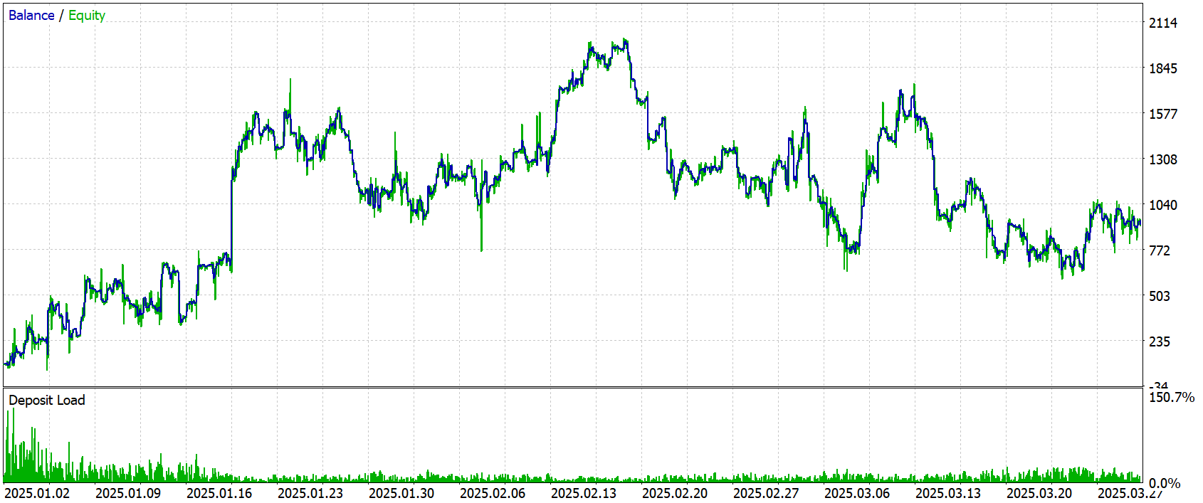
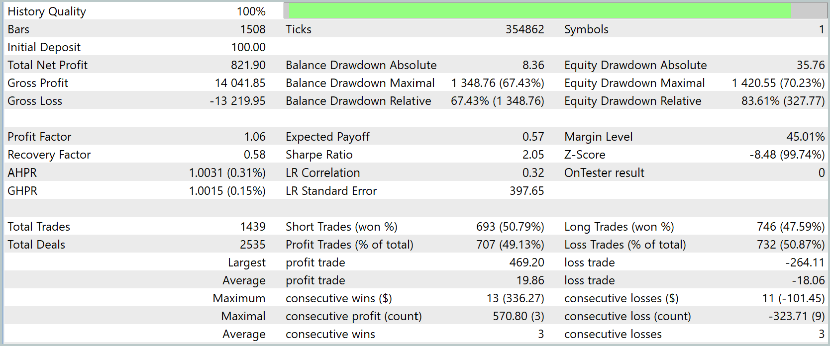
The test results show that the model returned a profit over the selected historical period. Total net profit amounted to $821.90 on an initial deposit of $100.0, indicating capital growth. It should be noted, however, that the profitability ratio (Profit Factor) stands at 1.06, which indicates that profits only slightly exceed losses.

The trading metrics show that the number of profitable trades is roughly equal to the number of losing trades — about 49% and 51%, respectively — which indicates a balance between winning and losing positions.

The chart shows that the balance curve is generally rising, despite noticeable drawdowns and periods of decline. A clear upward trend in the account balance in January and the first half of February is particularly noteworthy. At the same time, March appears to be clearly loss-making. This may indicate the need to fine-tune the model on a longer segment of historical data.

Conclusion

In conclusion, we note that the proposed K²VAE framework, as part of our trading agent, has proven its viability and has been validated on real historical data. The model combines a deep understanding of underlying market dynamics, adaptive risk adjustment, and the generation of probabilistic scenarios, which made it possible to achieve capital growth. At the same time, the decline in performance over an extended testing interval indicates the need to find ways to improve the model's generalization capability.

References

• K²VAE: A Koopman-Kalman Enhanced Variational AutoEncoder for Probabilistic Time Series Forecasting
• Other articles in this series

Programs Used in This Article

#	Name	Type	Description
1	Study.mq5	Expert Advisor	Expert Advisor for offline model training
2	StudyOnline.mq5	Expert Advisor	Expert Advisor for online model training
3	Test.mq5	Expert Advisor	Expert Advisor for model testing
4	Trajectory.mqh	Class library	Structure for describing the system state and model architecture
5	NeuroNet.mqh	Class library	Class library for creating a neural network
6	NeuroNet.cl	Library	Code library for the OpenCL program