Neural Networks in Trading: Unraveling Structural Components (SCNN)

Introduction

Forecasting multivariate time series is a fundamental problem in machine learning. It is through this lens that a wide range of applied problems can be examined: from estimating demand and forecasting traffic to identifying the behavior of market participants and quote movements. This is particularly relevant in the financial sector — after all, virtually any asset, whether it is a stock, a currency, or a commodity, is represented by a complex multivariate time series with a multitude of interrelated factors: volumes, prices, indicators, macroeconomic data, behavioral signals, and so on.

The main challenge in making such forecasts is identifying spatiotemporal patterns. Spatial aspects are reflected in the characteristics of the external environment: differences in liquidity, trading sessions, and regional activity. Temporal patterns, on the other hand, are linked to the rhythms of the markets themselves — trading cycles, news-driven bursts, and the periodicity of macroeconomic data releases. In practice, financial time series are far from stationary. They are subject to abrupt changes, distribution shifts, and complex transitions between phases — trends, sideways markets, panic, and euphoria. Furthermore, autocorrelation dependencies are unstable: what works today may have no predictive power tomorrow.

Modern neural network-based methods, such as transformers, recurrent neural networks, and convolutional architectures, do not require the stationarity assumption and have proven effective in short-term forecasting tasks. However, in real-world market conditions, they most often demonstrate robustness only to familiar patterns. When faced with sudden shifts, however — whether a liquidity collapse or a change in the behavior patterns of market participants — their accuracy drops sharply. Furthermore, such models essentially remain black boxes with a high computational load and limited interpretability.

In this regard, the idea of decomposing time series — that is, breaking them down into trend, seasonality, and residual fluctuations — is attracting increasing attention. This approach simplifies the problem structure, improves the model's adaptability, and provides a clearer understanding of the basis for the forecast. Even simple linear models that use decomposition outperform complex neural networks in terms of accuracy and stability in some cases.

However, it is worth acknowledging that even these methods have their limitations. Many of them focus exclusively on long-term and seasonal components, ignoring short-term or volatile segments, which are precisely where the key market signals lie. Furthermore, processing different components separately, without any information exchange between them, makes it difficult to capture high-level and nonlinear interactions. However, the use of static parameters proves ineffective in the face of dynamic autocorrelation, since the model's optimal settings must adapt flexibly based on the current market conditions.

To overcome these challenges, the paper "Disentangling Structured Components: Towards Adaptive, Interpretable and Scalable Time Series Forecasting" introduced a new architecture — the Structured Component Neural Network (SCNN). It is the first neural network of its kind, built entirely on the structural decomposition of time series. The main idea behind SCNN is to strategically decompose data into several heterogeneous components: not only long-term trends and seasonal fluctuations, but also rapidly changing, volatile segments. Each group is processed by a dedicated subnetwork tuned to its own dynamics. Thanks to this approach, the model becomes more responsive to changes in market conditions, and its operation becomes more understandable and transparent.

A key distinguishing feature of SCNN is that the decomposition and reconstruction processes are integrated into the neural network structure itself, rather than being limited to the input and output stages. This architecture makes it possible not only to perform deep decomposition of the data, but also to identify complex interactions between components, including cross-connections and latent dependencies. Furthermore, each network module is built using a two-branch architecture: one branch dynamically adapts the model parameters to current market conditions, while the other uses these parameters to process hidden features. Essentially, the model reconfigures itself on the fly, adapting to the current autocorrelation structure.

To further improve the robustness and generalization capability of SCNN, the authors of the framework integrated a special structural regularization mechanism. This helps the model focus on those components of the time series that are less susceptible to noise and distortion. Thus, even in an unstable market environment, where some patterns quickly lose their strength while others emerge suddenly, SCNN maintains high accuracy and reliability.

This is corroborated by the results of extensive experimental testing conducted by the framework’s authors on three independent datasets. SCNN consistently outperformed competing methods, particularly in the presence of sharp distribution shifts and anomalies in the data. What is particularly important is that all of this is achieved with a reasonable computational load, making the model suitable for both local computations and integration into trading systems.

The SCNN Algorithm

In their work, the authors of the SCNN framework assume that a time series is formed in stages — from random perturbations to complex market structures.

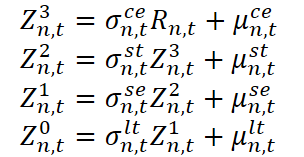
Here Z⁰n,t is the original value of the observed time series (for example, the price or trade volume), and Zⁱn,t for i = 1, 2, 3 are intermediate representations at different levels of the structure. Rn,t is the residual component, which includes noise or unexpected outliers. Each stage includes both a multiplicative coefficient σ, which reflects the scaling effect, and an additive shift µ, which corresponds to absolute adjustments.

To gain an intuitive understanding of this structure, we will consider an analogy with market data analysis. Let’s have a look at the price dynamics of an asset. The long-term component reflects fundamental shifts. This could be due to the impact of interest rates or structural changes in the economy. The seasonal component consists of recurring patterns associated with quarterly earnings reports, tax periods, or the behavior of major market players. The short-term component captures local fluctuations caused, for example, by news releases, increased trading activity, or temporary liquidity shortages. The co-evolving layer models synchronous market events — for example, when several stocks from the same sector react simultaneously to a common piece of macroeconomic news. The residual component consists of white noise or outliers caused, for example, by isolated high-volume orders or quote errors.

It is important to understand that, under real-world market conditions, the boundaries between these layers are quite fluid. For example, a sharp increase in trading volume for a particular stock may initially be perceived as an outlier, but if it continues, it becomes a short-term trend. If it persists for weeks, it eventually becomes part of the long-term structure. This evolution of patterns requires models to be flexible and able to adapt to the changing structure of the data.

Within this framework, each component has both a multiplicative and an additive effect. The multiplicative effect allows us to model proportional changes. The additive effect, on the other hand, reflects constant shifts, such as the persistent impact of corporate dividends or seasonal fees that do not depend on the current price level. It is precisely the combination of these two types of effects that allows market data to be modeled as realistically as possible. After all, in some cases the relative change is the key factor, while in others it is the absolute value.

The long-term component is used to identify stable structural patterns in the time series, such as steady growth in trading volumes or an expansion in market activity against the backdrop of an economic upturn. By pattern, we do not simply mean a chronological sequence, but rather the shape of the distribution of aggregated data — without reference to specific points in time. Thus, the long-term structure is determined by the statistical profile of data collected over an extended period spanning several seasonal cycles.

The idea is simple: combining observations from different seasons makes it possible to smooth out short-term fluctuations and obtain a clearer, less noisy estimate of persistent trends. This approach helps avoid overfitting to temporary anomalies, such as one-time spikes in volume or short-term corrections, and allows us to focus on fundamental market dynamics.

To implement this approach, a sliding window of length ∆ is used, which allows observations to be dynamically selected at each time step. Next, two key statistical parameters are calculated: the mean (or center of the distribution) and the standard deviation (which characterizes the scale of fluctuations). Both parameters are used together to form a representation of the long-term component. After that, each new segment being analyzed is normalized — the long-term mean is subtracted from it, and the result is divided by the standard deviation. This brings all segments to a common scale, eliminating long-term offsets and preparing the data for the next stage of decomposition.

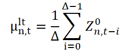
Here, μˡᵗn,t and σˡᵗn,t are, respectively, the long-term mean and scale (standard deviation) obtained from the data over the window ∆. Here, Z¹n,t is the normalized value with the long-term component removed, which is passed on to the next level of processing, where seasonality will be identified.

This stage can be interpreted as a leveled representation of the market, in which persistent structural trends have been accounted for. This is particularly important in financial forecasting, where short-term strategies (such as intraday strategies) require data that has been filtered to remove long-term shifts in order to identify local opportunities without distortion from global trends.

The seasonal component is responsible for identifying recurring cyclical patterns in a time series. In the context of financial markets, such patterns might include, for example, intraday peaks in trading activity: morning surges, a lull around lunchtime, and an evening ramp-up before the session closes. This could include weekly patterns — such as lower volatility on Fridays or higher trading volumes on Mondays — as well as quarterly and annual seasonal effects related to earnings reports or macroeconomic data releases.

It is assumed that the length of the seasonal cycle remains constant over time — this is a simplified but practical assumption. However, for scenarios with variable cycle lengths, the framework's authors suggest integrating automatic seasonality estimation using the FFT (Fast Fourier Transform).

Technically, the extraction of the seasonal component is organized similarly to long-term normalization, but with one important difference: a dilated window is used, with a step size that corresponds to the cycle length. Let τ be the window size, and m be the dilation factor (which is, in fact, the cycle length). This allows the data to be scanned at intervals that correspond to the seasonal structure.

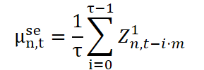
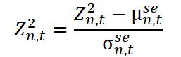
Here Z²n,t denotes the normalized, seasonality-adjusted data that are passed on to the next stage of processing.

The short-term component is responsible for capturing local and irregular deviations that cannot be explained by either long-term trends or seasonal patterns. In financial markets, such effects can be triggered by a sudden reaction to a news release, technical glitches, speculative surges in liquidity, or a sharp shift in trader sentiment amid volatility. This is a kind of market pulse that reflects the market's sensitivity to external stimuli over very short time intervals.

Unlike long-term normalization, a small smoothing window is used here to avoid blurring short-term fluctuations. Let δ be the length of this window. Based on this, standard statistical measures — the sample's location and scale — are calculated, after which the data are normalized.

The resulting value Z³n,t is an intermediate representation, filtered to remove short-term fluctuations, and is then passed on to the final stage of normalization.

However, this component has its limitations. First, it cannot react instantly to sudden, drastic changes — the model exhibits inertia. Second, if a change lasts only two or three time steps, it may go unnoticed, especially under conditions of high variance. This is similar to a market situation where short-term volatility in a single stock can be ignored by the system as a whole if its magnitude is lost in the aggregated noise.

To smooth out this effect and increase the model's sensitivity to short-term signals, SCNN includes the use of co-evolving time series. In other words, if a deviation is observed in one instrument, the model checks for synchronous signals in other assets, such as derivatives, indices, or trading volumes. Thus, the short-term component becomes not only reactive but also context-aware — which is particularly important in high-frequency and algorithmic trading.

The co-evolving component plays a special role in the overall structure of the model. Unlike the previous three components, which analyze the behavior of each time series in isolation, this part of the model relies on spatial correlations and makes it possible to capture instantaneous changes that occur simultaneously across multiple time series. If two or more time series exhibit similar dynamics at the same points in time, this strongly suggests the presence of a common generative process. In that case, we can estimate it by aggregating the relevant observations.

However, to implement this approach, a key challenge must be addressed: determining exactly which series are involved in this joint process. It boils down to measuring the correlation between time series. There are two possible approaches here: either fix the correlation matrix in advance based on expert knowledge, or learn it directly from the data. The authors of the framework chose the second approach — one that is more flexible and general-purpose, especially when there is no a priori information about the data structure.

For each pair of time series n and n', an individual attention coefficient is calculated, which is then normalized using the SoftMax function. This ensures that the sum of the weights for each series equals one.

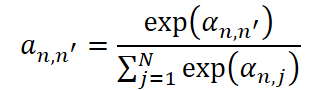
Using these weights, we calculate the parameters of the co-evolving component. First, the mean value is calculated, reflecting local centering while taking interrelationships into account.

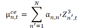
Next, the scale (standard deviation) is estimated with the addition of the stabilizing constant ϵ.

Based on this, a normalized residual is constructed.

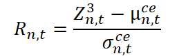
This residual Rn,t represents the portion of the signal that is not explained by any of the previously identified components. It reflects residual uncertainty, structural noise, or unique deviations of a specific series from the overall dynamics that are not amenable to formalization.

When working with a large number of time series, the model's scalability can be further improved. To this end, it is proposed to use an adjacency matrix learning module, which allows the attention architecture to be flexibly adjusted and computations to be optimized.

In the final stage, all intermediate representations are combined into a single feature vector.

At the same time, an auxiliary vector of normalization parameters is generated.

Thus, a time series is no longer simply a set of values recorded over time. It is transformed into a multicomponent representation in which each component accounts for a specific type of dynamics: a structural trend, recurring seasonal oscillations, local short-term fluctuations, or collective synchronous changes. This makes it possible to analyze data more accurately, build interpretable models, and develop robust forecasting algorithms.

Since each component exhibits its own dynamics with varying degrees of predictability, there is a natural need to model their behavior separately. This is particularly relevant for short-term forecasting, when long-term and seasonal components generally remain stable and follow fairly regular patterns. Under such conditions, they can continue to be extrapolated directly, without the need to introduce additional parameters or complex models.

Thus, for the long-term component, the simplest approach is used: it is assumed that its values remain constant throughout the entire forecast horizon. In other words, if the current estimates of this component's parameters are known, we simply carry them forward into the future.

The seasonal component, on the other hand, is based on periodicity and requires a slightly more nuanced approach. Since the cyclicity is preserved, we reuse parameter values from past time points that are in the same phase of the cycle as the point being forecast. In other words, the values of the seasonal component at time t+i are taken from time t-m+i, where m is the cycle length.

This method preserves the seasonal rhythm and allows the component's behavior to be extrapolated with high accuracy without placing an additional burden on the model.

Unlike the long-term and seasonal components, the short-term component, co-evolving dependencies, and residual representations exhibit much greater stochasticity. Their dynamics are significantly less regular, which makes it impossible to use fixed heuristics or rigidly defined extrapolation rules. For this reason, for each of these three components, the framework’s authors apply a parameterized model based on autoregression; this allows them to account for their complex and unpredictable fluctuations.

For each time point i within the forecast horizon, the values of the corresponding components are calculated based on the previous δ values, using a linear model with trainable weights. The extrapolation procedure is the same for the short-term, co-evolving, and residual components, and is expressed as follows:

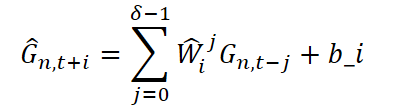
where G ∈ {Zˡn,t+i, μ^stn,t+i, σ^stn,t+i,μ^cen,t+i, σ^cen,t+i} denotes the extrapolated parameters corresponding to the various components; Ŵ^ji ∈ R^{dz · dz} are trainable weight matrices reflecting the contribution of past values; bi is the bias term (bias), which is also trainable.

After extrapolation, all components are combined into two vectors:

• Ĥn, t+i — a set of statistical parameters;
• Źn, t+i — a set of normalized representations.

To model the interaction between these two sets of features, pairwise multiplication (an element-wise product) is applied to two linear projections, each of which is formed using a trainable parameter matrix.

Thus, the final forecast representation is formed, synthesizing all statistically significant aspects of the process under study.

Implementation Using MQL5

After a detailed examination of the theoretical foundations of the SCNN framework, we move on to its practical implementation. This section presents one practical implementation option for bringing the model's key ideas to the application level using MQL5. We will demonstrate how to decompose a time series into its structural components and how to build the predictive part of the model while preserving its interpretability and modularity. This approach paves the way for creating intuitive, flexible, and adaptive trading strategies based on complex neural network architectures.

At the first stage of implementing the SCNN framework, we will focus on building the core block: an algorithm for extracting statistical characteristics and normalizing input data within fixed time intervals. This stage plays a key role in decomposing the time series, since it is here that the long-term and short-term components are formed, on which all subsequent forecasting will later be based.

The algorithm is implemented as an OpenCL kernel named PeriodNorm, which is responsible for calculating statistical characteristics and normalizing data within sliding windows of the time series. The implementation is based on the concept of parallel processing, in which data for all variables and time windows are processed simultaneously.

__kernel void PeriodNorm(__global const float* inputs,
                         __global float2* mean_stdevs,
                         __global float* outputs,
                         const int total_inputs
                        )
  {
   const size_t i = get_global_id(0);
   const size_t p = get_local_id(1);
   const size_t v = get_global_id(2);
   const size_t windows = get_global_size(0);
   const size_t period = get_local_size(1);
   const size_t variable = get_global_size(2);

The function takes an array of input values, inputs, as well as arrays for storing normalized values, outputs, and the calculated statistical parameters (means and standard deviations), mean_stdevs. The total_inputs parameter is also passed; it defines the length of the time series per variable.

The work-items are organized in three dimensions: the first coordinate corresponds to the window number (time segment), the second to the position within the window, and the third to the variable index. Thus, each work-item is responsible for one specific time series element within a specific window and for a specific variable.

First, the indices required for proper access to the data in memory are calculated. The variable shift_i specifies the position of the current point relative to the start of the time series, shift_v specifies the offset across variables, and shift_ms specifies the position in the statistics array.

   __local float Temp[LOCAL_ARRAY_SIZE];
   const int shift_i = i * period + p;
   const int shift_v = v * total_inputs;
   const int shift_ms = v * windows + i;

After that, the time series value is retrieved from the source array while checking for invalid values: if NaN or infinite values are encountered, they are replaced with zero.

//---
   float val = 0;
   if((shift_i) < total_inputs)
      val = IsNaNOrInf(inputs[shift_v + shift_i], 0);

The next step is to compute the mean value within the current window. For this, the LocalSum helper function is used; it sums element values across the work-items in the local group, which significantly improves performance.

   float mean = IsNaNOrInf(LocalSum(val, 1, Temp) / period, 0);
   val -= mean;
   BarrierLoc;

The resulting mean is then subtracted from the current observation, and the standard deviation is calculated on this basis as the square root of the mean squared deviations. All stages include built-in numerical stability checks to prevent division by zero and the accumulation of errors.

   float stdev = LocalSum(val * val, 1, Temp) / period;
   stdev = IsNaNOrInf(sqrt(stdev), 1);

The results are stored in two forms: first, the statistics for each window and variable are written to the mean_stdevs array, and second, the normalized values are returned in the outputs array.

   mean_stdevs[shift_ms] = (float2)(mean, stdev);
   if((shift_i) < total_inputs)
      outputs[shift_v + shift_i] = IsNaNOrInf(val / stdev, 0);
  }

Normalization is performed using the classic z-score normalization formula, with the standard deviation calculated on the fly used as the norm.

The kernel is designed to scale easily: you can change the window size, the number of variables, or the length of the time series without altering the logic. In particular, as the window length increases, normalization becomes sensitive to long-term trends and can be used to extract the trend. Conversely, reducing the window size allows for more accurate detection of short-term deviations and anomalies.

To implement a model with a full training cycle that includes backpropagation, we need to ensure that gradients can be propagated from the outputs of the neural network architecture to its inputs. Although the PeriodNorm kernel has no trainable parameters (all computations are strictly statistical and based on the input time series data), gradients must be computed if normalization is performed as part of the computational graph. Therefore, we add a second kernel, PeriodNormGrad, to the architecture.

__kernel void PeriodNormGrad(__global const float* inputs,
                             __global float* inputs_gr,
                             __global const float2* mean_stdevs,
                             __global const float2* mean_stdevs_gr,
                             __global const float* outputs,
                             __global const float* outputs_gr,
                             const int total_inputs
                            )
  {
   const size_t i = get_global_id(0);
   const size_t p = get_local_id(1);
   const size_t v = get_global_id(2);
   const size_t windows = get_global_size(0);
   const size_t period = get_local_size(1);
   const size_t variable = get_global_size(2);

Unlike classical blocks with trainable parameters, the algorithm implemented in the PeriodNormGrad kernel is designed to correctly propagate the error backward through a layer that itself contains neither neurons nor weights. First, element-wise access to each time window of the series is set up inside the kernel for each variable. The indices are calculated in the same way as in the forward pass:

• i — window number,
• p — position within the window,
• v — variable number.

After obtaining the coordinates in this way, we extract all the required data: the input value (inp), its normalized version (out), the error gradient with respect to the normalized value (out_gr), as well as the precomputed mean and standard deviation for the window (mean_stdev) and the gradients with respect to them (mean_stdev_gr), which can also be obtained when the values are used repeatedly. In particular, the SCNN framework assumes they will be used for data extrapolation. All values are checked for validity — NaN values and infinities are filtered out to avoid corrupting the calculations.

   __local float Temp[LOCAL_ARRAY_SIZE];
   const int shift_i = i * period + p;
   const int shift_v = v * total_inputs;
   const int shift_ms = v * windows + i;
//---
   float inp = 0;
   float inp_gr = 0;
   float out = 0;
   float out_gr = 0;
   const float2 mean_stdev = means_stdevs[shift_ms];
   const float2 mean_stdev_gr = means_stdevs_gr[shift_ms];
   if((shift_i) < total_inputs)
     {
      inp = IsNaNOrInf(inputs[shift_v + shift_i], 0);
      out = IsNaNOrInf(outputs[shift_v + shift_i], 0);
      out_gr = IsNaNOrInf(outputs_gr[shift_v + shift_i], 0);
     }

Now for the most interesting part. To understand how much each input value affected the model's final error, we need to calculate how the error would change if that value were changed slightly. In statistics, normalization is performed by subtracting the mean and dividing by the standard deviation. This means that any change in the input will affect both the numerator (the deviation from the mean) and the denominator (the degree of dispersion within the window). Therefore, we need to calculate the gradients with respect to both parameters — the mean and the standard deviation.

   float mean_gr = LocalSum(out_gr, 1, Temp) / period + IsNaNOrInf(mean_stdev.x, 0);
   BarrierLoc;
   float stdev_gr = out * LocalSum(IsNaNOrInf(out * out_gr, 0), 1, Temp) / period +
                                                        IsNaNOrInf(mean_stdev.y, 0);

To do this, we first take the sum of all gradients at the layer output level, out_gr, over the current window and average it — this is the contribution to the gradient with respect to the mean (mean_gr). Note that here we are not simply passing the gradient directly: we are taking into account how a change in the mean affects the normalized values across the entire window.

Next, calculating the gradient with respect to the standard deviation (stdev_gr) is a bit more complicated: here, we multiply the mean-adjusted value by its error gradient, then average the result, thereby obtaining the sensitivity of the error to the dispersion of the data.

Now that we have both of these gradients, we can move on to calculating the main result — the gradient with respect to the input itself. We combine the gradient from out_gr with the derivatives with respect to the mean and standard deviation. The final formula is balanced and makes it possible to accurately reflect the contribution of each input value to the model’s total error, taking into account its position within the window and its impact on the overall statistical characteristics.

   inp_gr = (out_gr - mean_gr - stdev_gr) / IsNaNOrInf(mean_stdev.y, 1);
//---
   if((shift_i) < total_inputs)
      inpurs_gr[shift_v + shift_i] = IsNaNOrInf(inp_gr, 0);
  }

Finally, as usual, the resulting value is written back to the input-gradient array (inputs_gr). All operations take the array bounds into account: if the current index falls outside the array bounds, no operations are performed.

Thus, PeriodNormGrad is not merely a formal implementation of gradients, but an important functional bridge between classical statistics and modern model training methods. It allows statistical operations to be full-fledged participants in the computational graph and to take part in training, correctly passing error information back to where it originated.

In the main program, we will create a specialized class, CNeuronPeriodNorm, designed to encapsulate the logic for working with OpenCL kernels for period normalization, for both the forward and backward passes. It inherits from the base class CNeuronBaseOCL, which indicates that it belongs to the computational model's component hierarchy. The structure of the new object is shown below.

class CNeuronPeriodNorm :  public CNeuronBaseOCL
  {
protected:
   uint                    iPeriod;
   uint                    iVariables;
   uint                    iCount;
   CNeuronBaseOCL          cMeanSTDevs;
   //---
   virtual bool      feedForward(CNeuronBaseOCL *NeuronOCL) override;
   virtual bool      updateInputWeights(CNeuronBaseOCL *NeuronOCL) override { return true; }
   virtual bool      calcInputGradients(CNeuronBaseOCL *NeuronOCL) override;

public:
                     CNeuronPeriodNorm(void) : iPeriod(-1), iVariables(1) {};
                    ~CNeuronPeriodNorm(void) {};
   //---
   virtual bool      Init(uint numOutputs, uint myIndex, COpenCLMy *open_cl,
                          uint units_count, uint period, uint variables,
                          ENUM_OPTIMIZATION optimization_type, uint batch);
   //---
   virtual bool      Save(const int file_handle) override;
   virtual bool      Load(const int file_handle) override;
   //---
   virtual int       Type(void) override const  {  return defNeuronPeriodNorm; }
   virtual void      SetOpenCL(COpenCLMy *obj) override;
//---
   CNeuronBaseOCL*   GetMeanSTDevs(void) { return cMeanSTDevs.AsObject(); }
   virtual uint      GetPeriod(void) const { return iPeriod; }
   virtual uint      GetVariables(void) const { return iVariables; }
   virtual uint      GetUnits(void) const { return iCount; }
  };

The class's internal fields reflect key configuration parameters. Specifically, the variable iPeriod specifies the length of the window within which statistical processing — the calculation of the mean and standard deviation — is performed. The iVariables parameter specifies the number of variables (or features) to be processed, and iCount specifies the number of independent windows for each single sequence.

In addition, the class contains the cMeanSTDevs object, which serves as an intermediate buffer for storing the mean and standard deviation values calculated during the forward pass. This buffer also participates in backpropagation, as implemented in the PeriodNormGrad kernel.

The Init method acts as an initialization constructor — it receives all the parameters as input, uses them to prepare the internal structures, and binds the object to the necessary OpenCL resources.

The forward and backward pass methods essentially serve as utility wrappers. Their task is not to recompute the data manually, but to prepare everything needed to correctly enqueue the corresponding OpenCL kernels for execution.

Note the GetMeanSTDevs function — it provides access to a buffer containing computed statistics, which can be used by other components of the model, for example, for visualization or further processing.

Thus, the CNeuronPeriodNorm class is a fully autonomous and flexible component that not only performs normalization but also ensures proper integration into the structure of a computational model with training support. Everything is implemented strictly in accordance with the principles of neural network frameworks, while maintaining the clear logic characteristic of systems with manual computation control, such as MQL5 + OpenCL.

The complete code for this class, including its methods, is provided in the attachment for independent study.

Today we have done substantial and productive work. The material is quite dense and requires some time to digest. Now is the perfect time to take a short break, catch your breath — and then continue our work in the next article with renewed energy.

Conclusion

In this article, we explored the theoretical aspects of the SCNN framework, which offers an original and conceptually sound approach to decomposing time series into interpretable components: long-term, seasonal, short-term, and residual components. This structure not only improves forecasting accuracy but also significantly enhances the model's transparency, making its behavior more predictable and adaptable to changing market conditions.

Particular emphasis is placed on the differences in the dynamics of each component, which necessitates the use of specialized interpolation methods: simple repeating patterns are applied to the long-term and seasonal components, while short-term and residual fluctuations are modeled using trainable autoregressive structures.

In the practical section of this article, we began implementing our own interpretation of the proposed approaches and built one of the model’s basic elements — an algorithm for normalizing periodic segments of a time series. We examined the details of implementing computations on the OpenCL side, including forward and backward passes, which will subsequently allow us to integrate this mechanism into a trainable neural network architecture. This step was a key milestone in the practical adaptation of the framework for trading tasks in the MQL5 environment.

In the next article, we will continue to develop this implementation by adding new model components and gradually moving toward a full-fledged system for analyzing and forecasting time series based on the SCNN framework.

Links

• Disentangling Structured Components: Towards Adaptive, Interpretable and Scalable Time Series Forecasting
• Other articles in the series

Programs used in this article

#	Name	Type	Description
1	Study.mq5	Expert Advisor	Expert Advisor for offline model training
2	StudyOnline.mq5	Expert Advisor	Expert Advisor for online model training
3	Test.mq5	Expert Advisor	Expert Advisor for model testing
4	Trajectory.mqh	Class library	Structure for describing the system state and model architecture
5	NeuroNet.mqh	Class library	Class library for creating a neural network
6	NeuroNet.cl	Library	Code library for an OpenCL program