Neural Networks in Trading: The Adaptive Graph Diffusion Model (SAGDFN)

Introduction

Multivariate time series are characterized not only by the familiar temporal dependence (trends, seasonality, sudden spikes in activity), but also by spatial correlation, which is far more insidious. It describes how changes in one sequence affect others. And these connections take on a life of their own: they appear and disappear, and their strength and direction change depending on global news, shifts in national monetary policy, political crises, or technological breakthroughs. For example, the EURUSD exchange rate may fluctuate in response to changes in natural gas prices in Europe caused by energy shocks, while the stock prices of semiconductor manufacturers may be affected by conditions at Asian factories.

Traditional models like ARIMA or VAR worked reasonably well with individual time series, but as soon as you are dealing with hundreds of instruments, they start to struggle. Next-generation machine learning methods (support vector machines (SVMs), Gaussian processes) have expanded the horizons of analysis, but their architecture has rarely taken into account the rich network of interconnections. Even modern recurrent neural networks (RNNs) and transformers, which have demonstrated impressive results in sequence processing, have proven to have limitations in a multivariate context: they lacked the flexibility needed to handle dynamic correlation networks.

Against this backdrop, graph neural networks (GNNs) emerged; they were originally designed for tasks with a distinct graph structure: transportation networks, social interactions, and supply chains. But in the world of finance, constructing such a graph is a task bordering on art. Two companies in the same industry may behave in completely opposite ways, while two distant markets (such as the U.S. and Japan) may react in unison to the same macroeconomic stimuli.

The solution was adaptive-weight graph neural networks (adaptive-weight GNNs), which construct a graph directly from the data rather than from assumptions. They train a matrix of relationships between assets, identifying real correlations rather than formal ones. A classic example: gold and the Japanese yen, which often behave as safe-haven assets. Under normal circumstances, the connection between them may not be obvious, but during periods of global upheaval, the model will detect the synchrony in their movements and adjust the forecast accordingly.

Nevertheless, even these approaches are not without their limitations. First, scalability: an N×N correlation matrix for a large number of assets turns into a resource-hungry monster that can bog down even powerful GPUs by flooding their memory with intermediate calculations. Second: spurious connections. Many adaptive algorithms assume that all nodes are connected to some extent, but this is not the case. In financial forecasts, a minor stock on a local market should not have a significant impact on global forecasts.

To address these problems, a new approach was developed based on graph diffusion and the principle of spatial sparsity. The key is not to try to analyze every possible connection, but to identify key nodes — anchors of influence of sorts — that set the tone for the entire system. In a financial context, these could include the U.S. dollar, the euro, oil, gold, and the S&P 500 and Nikkei 225 stock indices.

Among such algorithms, the SAGDFN framework stands out; it was presented in the paper "SAGDFN: A Scalable Adaptive Graph Diffusion Forecasting Network for Multivariate Time Series Forecasting". The framework's authors suggest selecting the most significant nodes using the Significant Nodes Sampling algorithm. The Sparse Spatial Multi-Head Attention module is then used to further refine these interdependencies. The result is a compact N×M matrix, where M is many times smaller than N.

Using the proposed approach reduces computational complexity from N² to MN while also reducing memory consumption. It enables forecasts to be generated for massive datasets without overloading computing resources and makes the system more robust to noise. This becomes particularly important during periods of market turbulence caused by unexpected decisions by central banks and sharp fluctuations in commodity prices.

The practical implications are clear. Large investment funds gain a tool for more precise portfolio rebalancing. For hedge funds, it provides a basis for strategies that account not only for the dynamics of individual assets but also for the complex interplay of global interdependencies. Algorithmic traders gain the ability to work with a large number of instruments without critical delays in decision-making.

The SAGDFN Algorithm

The Scalable Adaptive Graph Diffusion Forecasting Network (SAGDFN) is a state-of-the-art algorithm designed to make time-series forecasting more flexible, scalable, and efficient, even when working with extremely large graphs. The main idea is to significantly reduce the computational load and memory requirements without compromising the accuracy of the forecasts. Instead of mechanically processing the entire graph structure, the model focuses on the most significant elements and connections that have a real impact on the final result. This approach not only eliminates excess noise but also makes it possible to generate forecasts more quickly, cost-effectively, and accurately.

In the operation of SAGDFN, the α-Entmax function plays a crucial role. It acts as a kind of filter that helps the model identify truly important spatial correlations between the nodes of a graph and ignore secondary connections. This is particularly valuable in situations where the data have a complex and dynamically changing structure, such as in financial markets or urban transportation systems. Based on the selected connections, a compact adjacency matrix is formed; this matrix is not specified manually but is generated during the training process. This dynamic construction makes the algorithm more flexible and better able to adapt to new conditions without requiring a complete reconfiguration.

The SAGDFN architecture is based on the time-tested Encoder-Decoder framework, yet it does not require any prior knowledge of spatial relationships. This ensures the model’s versatility and its applicability across a wide range of fields: from the analysis of financial fluctuations — where it is important to identify the interrelationships among a multitude of assets — to the forecasting of energy flows, logistics routes, and even production chains. The model sequentially identifies the most significant neighbors of each node, combines them with the initial information, and constructs a dense adjacency matrix, which is then used for spatiotemporal analysis.

A distinctive feature of SAGDFN is that all of its key components are trained synchronously and in a coordinated manner. In a unified optimization loop, the indices of significant nodes, their embeddings, the attention parameters, and the final adjacency matrix are optimized. The L1 loss function is used during training; it helps balance prediction accuracy and robustness to noise in the data. This approach ensures that, over time, the model not only improves the quality of its forecasts but also adapts to changes in the structure of the system being analyzed.

Consequently, SAGDFN solves one of the long-standing problems in graph neural networks: how to maintain high prediction accuracy while avoiding excessive complexity and computational overhead.

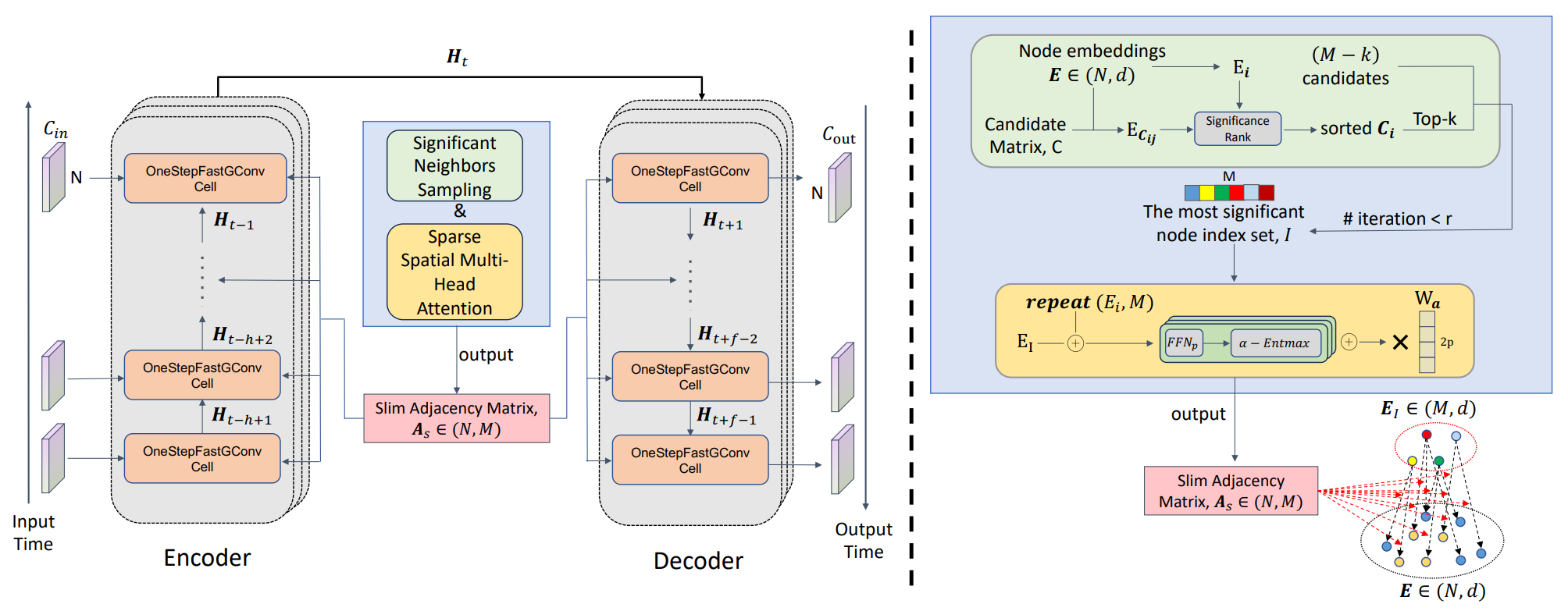
The authors of the SAGDFN framework assigned the task of selecting the most significant nodes to the Significant Neighbors Sampling (SNS) module — a methodological approach aimed at optimizing computational processes in graph neural networks (GNNs) when predicting time series with a large number of interconnected elements.

Traditional implementations of graph models construct a full N×N adjacency matrix and use it for subsequent graph convolution to identify spatial correlations among all nodes in the graph being analyzed. However, this approach has quadratic computational complexity, which makes it extremely resource-intensive. This is especially true when the number of nodes exceeds 2000 — a situation often encountered in real-world applications, whether in financial markets, transportation networks, or industrial monitoring systems.

The main idea behind SNS is to rethink the importance of connections: not every node has a significant impact on the state of a particular element in the graph. To make an accurate prediction, it is sufficient to consider only a small, highly relevant subset of neighbors that make a key contribution to the dynamics of the process. The method proposes dynamically selecting such significant neighbors from among all N nodes, creating a compact adjacency matrix of size N×M, where M is significantly smaller than N. This reduces the load on computational resources and speeds up data processing, while maintaining the model's ability to accurately reflect the system's internal relationships.

The operation of SNS begins with initializing the node embedding matrix E ∈ R^N×d, where each row Ei is a vector representation of the i-th node and contains information about its characteristics and relationships. At the same time, a candidate matrix C ∈ {1,…,N}^N×M is constructed, where each row specifies a set of potentially significant neighbors for the corresponding node. At this stage, it has not yet been determined exactly which neighbors will prove to be the most important — the selection problem is solved later, taking into account the spatial and contextual characteristics of the data.

Next, the SNS algorithm ranks the M candidates for each node according to their significance, using a proximity measure between embeddings — most often Euclidean distance, although other metrics may also be used. The smaller the distance between the vector representations of two nodes, the higher the probability that their relationship truly reflects the actual influence of one on the other. After that, a final set of the K most significant neighbors is formed, which serves as the core of the adjacency matrix. The remaining M−K positions can be filled with randomly selected elements to increase the diversity of connections and improve the model's robustness to local fluctuations in the data. This combined approach avoids excessive structural rigidity and prevents overfitting, which often occurs when connections are statically fixed.

The method outputs an index set I of significant nodes, from which a compact adjacency matrix As of size N×M is constructed. This approach significantly reduces computational complexity, bringing it close to linear instead of the conventional quadratic O(N²) implementation. And it does so without sacrificing forecast quality. As a result, SNS opens up the possibility of applying graph neural networks in areas where such approaches were previously considered too resource-intensive: it is possible to predict, in real time, fluctuations in market prices, the distribution of traffic flows, changes in energy consumption, and other processes where the interrelationships between elements play a decisive role.

Thus, Significant Neighbors Sampling does more than just conserve resources — it allows us to rethink the very concept of working with large graphs. Moving away from a global analysis of all relationships in favor of dynamic and selective analysis creates the conditions for building more flexible and adaptive predictive models that learn to focus on what really matters, rather than getting bogged down in excessive data.

The sparse spatial multi-head attention module (Sparse Spatial Multi-Head Attention) in SAGDFN is the core component that transforms the selected significant neighboring nodes into a compact connection matrix As of size N×M, which determines how much information should flow from each of the M nodes to a specific node i during graph convolution. Unlike approaches based on prior knowledge of topology, the SS-MHA module is built entirely from data. It does not rely on external structures and is not susceptible to erroneous or outdated assumptions about spatial relationships. This makes the model versatile and applicable to a variety of problems in financial markets, energy grids, or traffic flows, where the relationships between components change over time and cannot be captured by a simple hand-crafted model.

Technically, the module combines two key concepts. First, the inner product of vectors allows for an efficient and parallel estimation of a basic measure of similarity between nodes: the vector of node i is transformed into an M×d matrix by repeating the row and concatenating it with the embeddings of its M significant neighbors. This creates a matrix that simultaneously contains information about a node’s local context and its candidate neighbors, paving the way for fast matrix operations in modern automatic differentiation frameworks.

Second, the authors of the SAGDFN framework depart from a purely linear approach and train a nonlinear correlation measure using small Feed-Forward neural blocks (FFNs). For each node and each attention head, these FFNs transform the concatenated representations into a score matrix Y, where the two columns are interpreted as probable and less probable correlations, respectively. In this context, a multi-head architecture resembles the work of a group of experts examining the same dataset from different angles: one head identifies seasonal relationships, another detects reactions to news, and a third uncovers latent risk indicators.

A key step is the normalization of scores. Instead of the standard SoftMax, which spreads the weights across the entire set and often creates many small, insignificant connections, the framework's authors suggest using the α-Entmax function. It produces sparse but informative attention distributions: large values are amplified, while small ones are suppressed to zero. In financial applications, this is critical: there are only a few instruments in the market that are truly setting the direction at any given moment — a reserve currency, a major index, or a key commodity. α-Entmax acts like a lens that focuses on prominent objects and filters out background noise. The α parameter provides flexibility: it ranges from SoftMax (α=1) to SparseMax (α=2). The optimal degree of sparsity is selected for the specific data domain.

In practice, normalized scores Z^p are computed for each attention head, and these are combined into a multidimensional tensor Zi for node i. Next, a tensor Z of size N×M×(2P) is assembled over all nodes and, using a linear transformation with weights Wa, is reduced to the final matrix As of size N×M. This matrix is no longer a dense N×N graph; instead, for each node, it carefully selects only those M signals that actually influence the subsequent graph convolution.

This approach is particularly effective in financial markets, where instruments that influence price movements today may not have the same effect tomorrow. For example, during a period of panic, gold and the yen may be the leaders; during a phase of economic growth, the S&P 500 index and technology stocks may lead; and during an energy shock, oil prices and the currencies of energy-exporting countries may lead. The module makes it possible to identify such obvious and hidden leaders while ruling out random correlations that could distort the forecast.

In addition to improving forecast accuracy, α-Entmax offers other advantages: sparse scores reduce the number of unnecessary operations in graph convolution, making the model more interpretable; analysts can see which M nodes actually influenced the forecast for a specific instrument. The combination of random substitution when selecting neighbors and sparse normalization ensures that embeddings are updated across the entire network without overlooking important variables.

The technical implementation takes into account the efficient use of GPUs and automatic differentiation frameworks: concatenation and batch processing, compact FFNs for each head, and a linear transformation of the final tensor Z into As for fine-grained parameterization of the influence of each head and each channel.

Taken together, Sparse Spatial Multi-Head Attention provides a practical trade-off between accuracy and resource efficiency: sensitivity to the most important signals, adaptability to changing conditions, and scalability to thousands of time series.

Forecasting based on the Encoder–Decoder architecture in the SAGDFN framework is the culmination of all previous stages. This approach combines previously selected significant neighbors, sparse spatial multi-head attention, and efficient graph convolution with a powerful sequential model that makes it possible to account for temporal dynamics. Unlike simpler approaches that focus on spatial dependencies or the temporal aspect, the approach proposed by the framework authors makes it possible to describe and use both dimensions jointly. This provides more accurate and robust forecasts for multivariate time series.

Intuitively, the operation of Encoder–Decoder can be viewed as follows. The Encoder condenses information from the historical sequence, accumulating spatiotemporal patterns in a compact representation of hidden states. The Decoder then generates forecasts step by step, using this representation and the forecast values received at each step.

In this case, the critical component is a fast graph diffusion mechanism based on the compact adjacency matrix As, which ensures the transmission of relevant information between graph nodes at each time iteration.

A multi-step graph convolution that implements information diffusion among neighbors is defined by the expression:

where D is the diagonal degree matrix for As, IN is the identity matrix of size N, and XI is the matrix of input data aggregated over the selected M neighbors (indexed by I).

Such an operator preserves information about the node’s own state (the X term) and accumulates the signal from relevant neighbors (AsXI), then normalizes them by the degree sum and passes them through linear filters Wj. The practical benefit is the ability to control the radius of information propagation using the parameter J: a small J captures local connections, while a large one accounts for more distant influences.

Next, the authors of the SAGDFN framework integrate this graph operation into a GRU-like step, replacing standard matrix multiplication with graph convolution. This gives rise to OneStepFastGConv, a one-step iteration that combines spatial aggregation and temporal recurrence:

Here, the concatenation operator ⊕ combines the current observation with the previous hidden state, while the operators ⊙ and σ have their usual meanings. This step ensures that, before updating its hidden state, each node takes into account its own features and the signal from its most significant partners in the graph. This is particularly important in finance: when forecasting a stock’s price, not only the stock’s own history is considered, but also the movements of key related instruments — currencies, commodities, and indices.

Data forecasting is performed in two stages: the Encoder and the Decoder. In the Encoder, we run OneStepFastGConv on a historical window of length h, ultimately obtaining a representation Ht0-1 that accumulates the spatiotemporal information of the entire analyzed data window.

Then the Decoder starts with the initial state Ht0-1 and the observation at step t0, sequentially generating the specified number of future steps.

Training is performed using end-to-end backpropagation — gradients with respect to Θ (including embeddings, FFN parameters in the attention module, graph convolution weights, and GRU parameters) are computed and used to update the model. It is worth noting that, since embeddings are involved in both neighbor selection and the calculation of As, the graph structure also changes over the course of training: this gives the system adaptability, allowing it to discover new meaningful connections as the market changes.

The Encoder–Decoder, combined with OneStepFastGConv and the adaptive As structure, creates a powerful and flexible platform for spatiotemporal prediction. It combines interpretability (through a sparse connection matrix and the visualization of relevant neighbors), adaptability (dynamic updating of embeddings and graph structure), and practical scalability, making it a particularly valuable tool for analysis and decision-making in financial markets.

The authors’ visualization of the SAGDFN framework is shown below.

Implementation in MQL5

After a detailed discussion of the theoretical part of the SAGDFN framework, we move on to the practical implementation of the proposed approaches. Here, we will show one practical way to transfer the framework authors’ ideas to the MQL5 environment. In the course of this work, we will consider the following points:

• data preparation;
• storing and updating embeddings;
• sampling significant neighbors;
• the sparse attention mechanism;
• integrating fast graph convolution into recurrent logic.

Our goal is a functional, reproducible, and — most importantly — practical implementation suitable for real-world operation.

The Significant Neighbors Sampling module performs one simple yet extremely important task: it is responsible for selecting the leaders that truly shape the network's information landscape. Correct neighbor selection determines which signals will be amplified and which will remain background noise.

It should be noted here that the authors of the SAGDFN framework proposed ranking the M most significant neighbors obtained at the previous step to form a set of the K closest elements, which serve as the core of the adjacency matrix. The remaining M−K positions are filled with randomly selected elements to increase the diversity of connections. In our implementation, we decided to take it a step further and add parallel ranking of a random sample.

The idea is simple yet effective: instead of first selecting the K nearest candidates and then supplementing them with random elements, we create two pools — one of preselected candidates and one of random candidates. We then evaluate them simultaneously. The final sample includes the nodes from the combined pool that are truly closest in terms of embeddings, regardless of whether they were selected using a heuristic or at random. This combination of exploitation and exploration gives the model both stability and flexibility: it retains proven leaders while remaining open to identifying new centers of market influence.

We will move the technical implementation of this algorithm into the OpenCL context. To do this, we create a SignificantNeighborsSampling kernel.

__kernel void SignificantNeighborsSampling(__global const float *data,
                                           __global const float *candidates,
                                           __global const float *random_cands,
                                           __global float *neighbors,
                                           const int dimension
                                          )
  {
   const size_t main = get_global_id(0);
   const size_t slave = get_local_id(1);
   const int total_main = (int)get_global_size(0);
   const int total_slave = (int)get_local_size(1);

The kernel begins with a signature declaration. It takes as input the global arrays data, candidates, and random_cands, which are intended to store the series embeddings and the two candidate pools. The neighbors array is used to store the results. The integer dimension is responsible for the embedding size. The signature defines the scope of the work: one global work-item is responsible for one primary node (main), while a set of local work-items within a group is responsible for processing candidates.

Next, the execution context identifiers are extracted, local arrays are declared, and the working local size is calculated.

   __local int Idx[LOCAL_ARRAY_SIZE];
   __local float Temp[LOCAL_ARRAY_SIZE];
   const int ls = min(total_slave, (int)LOCAL_ARRAY_SIZE);

Local memory is a powerful tool for accelerating computation: here, it is used as a buffer for temporarily storing indices and distances within a subgroup.

In the next block, we determine the offsets in the flat source-data arrays to the required sequence elements.

   const int shift_main = RCtoFlat(main, 0, total_main, dimension, 0);
   int cand = (int)candidates[slave];
   int rand_cand = (int)random_cands[slave];

Next, it should be noted that we use two pools to search for the closest neighbors, one of which is generated by random sampling. In this case, it is quite likely that one or more elements of the sequence will be present in both samples. Therefore, the next block performs a simple duplicate check. This prevents the same index from being considered again, which is logical and saves computation. In the first step, we check for duplicates within the current work-item.

//--- duplicate check
   if(rand_cand == cand)
      rand_cand = -1;

Next, we check for duplicates among the set of previously selected neighbors.

//--- Look in candidates
   for(int l = 0; l < total_slave; l += ls)
     {
      if(slave >= l && slave < (l + ls))
         Idx[slave - l] = cand;
      BarrierLoc;
      for(int i = 0; i < ls; i++)
        {
         if(i >= (slave - l))
            continue;
         if(cand == Idx[i])
            cand = -1;
         if(rand_cand == Idx[i])
            rand_cand = -1;
        }
      BarrierLoc;
     }

Here, we write the candidates' indices to a local data array in batches, and then each work-item compares its indices with the elements of the array.

Please note that, to ensure that a single copy of each element is retained, we check only the indices of preceding work-items for duplicates. Consequently, only elements from subsequent work-items are excluded, while the element from the first occurrence is retained.

We then proceed in the same manner to check the pool of randomly selected candidates.

//--- Look in random candidates
   for(int l = 0; l < total_slave; l += ls)
     {
      if(slave >= l && slave < (l + ls))
         Idx[slave - l] = rand_cand;
      BarrierLoc;
      for(int i = 0; i < ls; i++)
        {
         if(i >= (slave - l))
            continue;
         if(cand == Idx[i])
            cand = -1;
         if(rand_cand == Idx[i])
            rand_cand = -1;
        }
      BarrierLoc;
     }

Once the candidates have passed the uniqueness check within the local group, we calculate the flat offsets shift_cand and shift_rand_cand to obtain the start of each candidate’s embedding in the data array.

   const int shift_cand = RCtoFlat(cand, 0, total_main, dimension, 0);
   const int shift_rand_cand = RCtoFlat(rand_cand, 0, total_main, dimension, 0);

Next, the calculation of the Euclidean distance begins. First, the local variables representing the distances of the candidates in both pools are initialized to zero.

//--- calc distance
   float dist_cand = 0;
   float dist_rand_cand = 0;
   for(int d = 0; d < dimension; d++)
     {
      float value = IsNaNOrInf(data[shift_main + d], 0);
      if(main != cand && cand >= 0)
         dist_cand += pow(value - IsNaNOrInf(data[shift_cand + d], 0), 2.0f);
      if(main != rand_cand && rand_cand >= 0)
         dist_rand_cand += pow(value - IsNaNOrInf(data[shift_rand_cand + d], 0), 2.0f);
     }

Next, in a loop over the embedding dimensionality, the values of the target embedding and the candidate embeddings are retrieved. To determine the distance, the squares of the differences between the target element and the corresponding candidate are summed in local variables.

It is worth noting that calculations are performed only for non-removed elements.

After calculating the distances, preparations begin for ranking the positions. First, we initialize the local variables cand_position and rand_position to zero, which corresponds to the first element of the array. However, we check whether the distances of elements from the preselected and random pools are equal. If the distances are identical, we give preference to the pool of previously selected candidates and increment rand_position.

//--- calc position
   int cand_position = 0;
   int rand_position = (int)(dist_cand >= dist_rand_cand);

This is followed by a series of blocks in which the current distances are collectively gathered from chunks of Temp local memory, and the number of elements in the local sample whose distance is less than the one under consideration is counted. The first series copies the distances from the pool of preselected candidates (or -1 for missing ones).

//--- by candidates
   for(int l = 0; l < total_slave; l += ls)
     {
      if(slave >= l && slave < (l + ls))
         Temp[slave - l] = (cand >= 0 ? IsNaNOrInf(dist_cand, -1) : -1);
      BarrierLoc;
      for(int i = 0; i < ls; i++)
        {
         if(i == (slave - l))
            continue;
         if(Temp[i] < 0)
            continue;
         if(cand >= 0)
           {
            if(Temp[i] < dist_cand)
               cand_position++;
            else
               if(Temp[i] < dist_cand && i < (slave - l))
                  cand_position++;
           }
         if(rand_cand >= 0)
           {
            if(Temp[i] < dist_rand_cand)
               rand_position++;
            else
               if(Temp[i] < dist_rand_cand && i < (slave - l))
                  rand_position++;
           }
        }
      BarrierLoc;
     }

Each work-item in the group iterates through the Temp elements, incrementing cand_position and rand_position depending on which distances are smaller. Subtle tie-breaking logic is used here: if two distances are equal, the order is determined by the index, which ensures deterministic ranking when distances are equal. Barriers ensure that Temp is properly filled before it is read and then cleared.

A similar second series does the same thing, but moves the distances of the random-sample elements into Temp and adjusts the positions once more, taking into account the remainder of the local subgroup.

//--- by random candidates
   for(int l = 0; l < total_slave; l += ls)
     {
      if(slave >= l && slave < (l + ls))
         Temp[slave - l] = (rand_cand >= 0 ? IsNaNOrInf(dist_rand_cand, -1) : -1);
      BarrierLoc;
      for(int i = 0; i < ls; i++)
        {
         if(i == (slave - l))
            continue;
         if(Temp[i] < 0)
            continue;
         if(cand >= 0)
           {
            if(Temp[i] < dist_cand)
               cand_position++;
            else
               if(Temp[i] < dist_cand && i < (slave - l))
                  cand_position++;
           }
         if(rand_cand >= 0)
           {
            if(Temp[i] < dist_rand_cand)
               rand_position++;
            else
               if(Temp[i] < dist_rand_cand && i < (slave - l))
                  rand_position++;
           }
        }
      BarrierLoc;
     }

It is important to understand this part: the algorithm implements distributed position counting — each slave independently determines where it will appear in the distance-sorted list of the local group. This gives us ranking without a global sort, entirely locally, which saves both memory and time.

The final step is to write the result. If a candidate exists and its position is less than the total number of neighbors being searched for, the offset index is calculated, and the candidate’s index is written to the corresponding cell of the neighbors array.

//--- result
   if(cand >= 0 && cand_position < total_slave)
     {
      const int shift_dist_cand = RCtoFlat(main, cand_position, total_main, total_slave, 0);
      neighbors[shift_dist_cand] = cand;
     }
   if(rand_cand >= 0 && rand_position < total_slave)
     {
      const int shift_dist_cand = RCtoFlat(main, rand_position, total_main, total_slave, 0);
      neighbors[shift_dist_cand] = rand_cand;
     }
  }

The presented algorithm performs a parallel evaluation of deterministic and random candidates, eliminates duplicates locally, computes distances, and ranks candidates by their position in the local subsample without global sorting.

We have done a great deal of substantial work today, and the article has already become quite thorough. Now is the perfect time to take a break, let our thoughts settle, and look at what we have done with a fresh perspective. In the next article, we will return to this topic with renewed energy and continue along the path we have begun, moving forward step by step.

Conclusion

In this article, we explored the SAGDFN framework, which stands out among similar solutions thanks to its scalability, its ability to work efficiently with large graphs, and its capacity to minimize computational costs without sacrificing accuracy. Its adaptive approach to selecting meaningful connections between nodes makes it possible to retain key information while avoiding overloading the model with unnecessary data.

In the theoretical section, we examined the framework's key features and internal mechanisms in detail. We explained how the algorithm works, and then took the first step toward implementing it. Particular attention was paid to the Significant Neighbors Sampling module, which plays an important role in optimizing computations and reducing costs when working with large graphs. At the same time, we made a number of improvements, making the neighbor-selection process more flexible and adaptive.

This work marked an important step toward the creation of a fully fledged predictive tool capable of effectively processing large amounts of data and extracting useful spatiotemporal dependencies from them. In the next article, we will continue in this direction, adding new components to the architecture and gradually moving toward comprehensive testing of the entire system on real historical data.

Links

• SAGDFN: A Scalable Adaptive Graph Diffusion Forecasting Network for Multivariate Time Series Forecasting
• Other articles in this series

Programs used in this article

#	Name	Type	Description
1	Study.mq5	Expert Advisor	Expert Advisor for offline model training
2	StudyOnline.mq5	Expert Advisor	Expert Advisor for online model training
3	Test.mq5	Expert Advisor	Expert Advisor for model testing
4	Trajectory.mqh	Class Library	Structure for describing the system state and model architecture
5	NeuroNet.mqh	Class Library	Class library for building a neural network
6	NeuroNet.cl	Library	Code library for an OpenCL program