Neural Networks in Trading: Adaptive Periodic Segmentation (Creating Tokens)

Introduction

In the previous article, we examined in detail the theoretical foundations of the LightGTS (Lightweight General Time Series Forecasting) framework — one of the most advanced and well-engineered approaches to time series forecasting today, which was presented in the paper "LightGTS: A Lightweight General Time Series Forecasting Model." Its concept is based on a deep understanding of the nature of periodicity characteristic of financial and economic data, as well as on a thoughtful reimagining of the Transformer architecture for the specific tasks of processing temporal structures. We focused primarily on how LightGTS handles periodic patterns, minimizing training costs and ensuring robust generalization even on heterogeneous and noisy data.

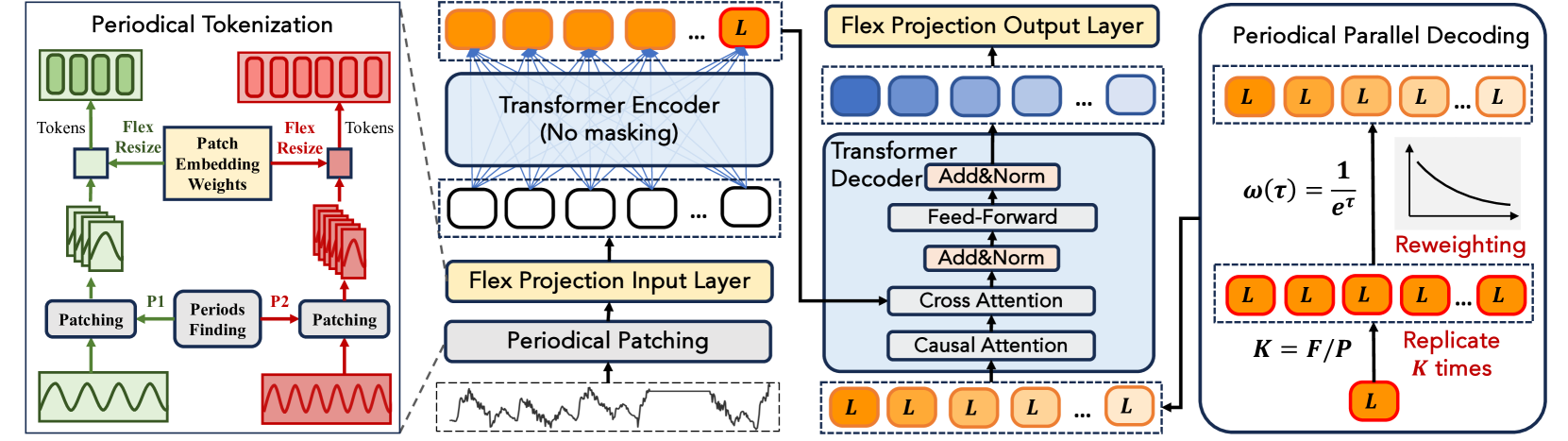
The framework begins with what is known as Period Patching — a mechanism in which a time series is divided into segments corresponding to the intrinsic frequency of the signal under analysis. This frequency is not set manually; it is determined by the model based on an analysis of the frequency spectrum obtained using the Fast Fourier Transform. Each extracted patch represents a single cycle containing significant local patterns. It is precisely this fragment that is converted into a token through projection. This is where the first architectural innovation comes into play — the Flex Projection Layer, which enables the processing of variable-length patches using a flexible linear transformation of the weights. This projection does not simply scale the data; it preserves the equivalence of tokens when moving between different scales and frequencies.

The Encoder block uses Rotary Positional Encoding (RoPE), which provides a compact and stable representation of the relative positions of tokens. This is especially important for financial series, where the absolute position is often much less significant than the relative positions of the elements within the sequence. The tokens are then processed by a classic stack of Transformer blocks, each of which consists of a multi-head Self-Attention module and a Feed-Forward module.

One of the most original solutions proposed by the authors of LightGTS was the Periodical Parallel Decoding mechanism, the conceptual opposite of autoregressive strategies. Instead of predicting the sequence step by step, the model uses the last token of the hidden representation (which encapsulates all the information about the previous sequence) and, based on this token, simultaneously generates the entire output sequence at once by replicating it and then applying positional weighting. This approach not only speeds up forecasting but also preserves periodic consistency in the temporal structure of the model output.

Finally, the framework applies Flex-resize to the Decoder's projection layer, thereby ensuring that the predictions match the actual length of the signal being forecast. All model training boils down to minimizing the classic MSE loss function between the predicted values and the target sequence.

Thus, LightGTS is not just a modified Transformer. This is a well-designed architecture in which each component is tailored to the specific characteristics of time series: from handling periodicity to moving away from autoregression in favor of fully parallel generation. It is precisely because of this deep adaptation that the framework achieves high accuracy with low computational cost.

The authors' visualization of the LightGTS framework is shown below.

In the practical section of the previous article, we began developing an algorithm for adaptive periodic patching — one of the key elements of the LightGTS architecture. The limitations associated with the inability to use dynamic memory allocation in the runtime environments typical of MQL5 and OpenCL were examined in detail. These limitations forced us to abandon the idea of an arbitrary number of output tokens.

Instead, we made a strategically sound decision: to fix the number of patches and use patch overlap as a tool to compensate for variations in the length of individual segments. Thus, we managed to strike a balance between adaptability (the model remains sensitive to the actual periodicity of the time series) and computational stability, which is necessary for the efficient use of hardware resources. This approach made it possible to preserve both the fidelity of representation of the cyclic structures in the analyzed data and predictability in memory management, which is critical for high-frequency trading models and for implementation in a constrained execution context.

We have already implemented the algorithm for selecting the dominant frequency: it effectively extracts the main periodicity for each univariate sequence in the input time series. This will allow us to specify a base scale for subsequent data segmentation. Today, we will continue the work we started and take the next step: implement the token generation algorithm within the OpenCL context.

Our goal is to divide each time series into a fixed number of segments, with the segment size determined according to the identified dominant frequency, while the overlap controls adaptation to the window length. All of this must be performed in a strictly parallel manner, using GPU-compatible code, where each thread (work-item) is responsible for generating a single token in one of the univariate components of the sequence being analyzed.

Building OpenCL Kernels

After identifying the dominant frequency using the fast Fourier transform, we have come right up to the key stage: building a mechanism for generating tokens, that is, time-series fragments that correspond to the identified periodicity. As a reminder, in the previous section we focused on an important task: combining the model’s adaptation to the current market frequency with the requirement for a fixed number of output patches, which is particularly important for running in the MQL5 environment, where dynamic memory allocation is unavailable.

Our approach is based on the following principle: the number of tokens (patches) remains constant, while their length is adjusted to the current frequency and the overlap is regulated to ensure complete coverage of the time series being analyzed. This allows for an effective balance between flexibility and resource control. However, there is a technical catch here: if the convolution window changes, then, logically, the weight matrix must also adapt — either by being rebuilt each time or by being projected onto a new space.

In the original paper, the authors of the LightGTS framework proposed a solution: the weight matrix is trained on a fixed window size (determined by the statistics of the training sample), and then, for each new window size, the weights are projected using the Moore–Penrose pseudoinverse. Mathematically elegant, but in practice — cumbersome.

Real financial markets are unforgiving: today's cycle is not tomorrow's cycle. Periodicity drifts, and adaptation requires flexibility. Computing the pseudoinverse matrix on the fly — especially in online processing or high-frequency trading — means sacrificing speed and resource efficiency for the sake of formal rigor. And that is an unaffordable luxury.

Our solution is much more practical. Instead of constantly rebuilding the weights, we took a different approach: we use a matrix of the maximum allowed size, in which we simply ignore unnecessary weights by using zero padding. In other words, if a data segment does not fall within the active window, it is multiplied by zero, and the corresponding weight has no effect on the result. Simple and effective.

This approach makes it possible to:

• maintain a fixed structure for the weight matrix, thereby avoiding computationally expensive operations;
• dynamically adjust the window size and the stride between patches;
• adapt to frequency fluctuations of the market on the fly, without stopping the model or recalculating its parameters.

All of this is implemented within the OpenCL context, in the FeedForwardAdaptConv kernel, where each work-item is responsible for a specific segment–filter pair for one of the univariate sequences.

__kernel void FeedForwardAdaptConv(__global const float *matrix_w,
                                   __global const float *matrix_i,
                                   __global float *matrix_o,
                                   __global const float *main_freq,
                                   const int inputs,
                                   const int window_in,
                                   const int activation
                                  )
  {
   const size_t u = get_global_id(0);
   const size_t f = get_global_id(1);
   const size_t v = get_global_id(2);
   const size_t units = get_global_size(0);
   const size_t filters = get_global_size(1);
   const size_t variables = get_global_size(2);

In the kernel body, we first determine the work-item indices in the three-dimensional task space. Next, using the univariate sequence identifier v, we retrieve the dominant frequency of the variable under analysis from the main_freq global buffer.

const int freq = main_freq[v];
int window = (inputs / variables + freq - 1) / freq;

From this, the window size is computed, with adjustments for the stride and fragmentation boundaries. Here, we also determine the stride of the analysis window based on the size of the input tensor and the number of tokens to be generated. The task is to cover the entire sequence evenly, with no omissions.

const int step = (int)(inputs / variables + units + 1) / (units + 2);
if(window < step)
   window = (int)((step + window - 1) / window) * window;
if(window > window_in)
   window = window_in;

Next comes the key point. It is important that the window is not smaller than the stride; otherwise, some of the data may not be covered. Therefore, if the detected period turns out to be too small, we increase the window size by a multiple, bringing it up to at least the stride without exceeding the maximum allowed value.

Next, the offsets in the input and output arrays, as well as in the weight matrix, are determined. This is necessary for correctly addressing data within the global buffers

const int shift_in = (u < (units - 1) ? u * step : inputs / variables - window);
const int shift_in_var =  v * inputs / variables;
const int shift_out = (u + v * units) * filters + f;
const int shift_weight = (v * filters + f) * (window_in + 1);

It is worth noting an important nuance here: we need to cover the entire input sequence, including its tail end. If segmentation is performed with a fixed stride and the length of each window is determined dynamically, the last few elements may be left out of the analysis. Therefore, to guarantee full coverage of the entire input sequence, we calculate the starting position of the last segment as the difference between the full length of the analyzed sequence and the window size. This allows the last window to be shifted so that it is guaranteed to capture the final data points of the sequence, even if its size was determined dynamically and turned out to be smaller than the maximum allowed size.

Next comes the main computational part — the convolution operation, during which the final value for each token is calculated. In the first step, we take the base value corresponding to the bias component, which is extracted from the weight matrix using a precomputed offset. This element serves as the starting point for accumulating the contribution from each element of the analysis window.

float sum = matrix_w[shift_weight + window_in];
for(int i = 0; i < window; i++)
   if((shift_in + i) < (inputs / variables))
      sum += IsNaNOrInf(matrix_i[shift_in_var + shift_in + i], 0) *
             matrix_w[shift_weight + i];

Next, we begin iterating through each element of the analysis window. This is where the key feature of our implementation comes into play — the zero-padding strategy. If an element of the sequence lies outside the actually computed window, it is simply excluded from the calculations. This helps prevent signal distortions that could occur if irrelevant data were included. This technique ensures consistent results and enables accurate calculations regardless of the current window size. In addition, zero padding makes it easier to maintain a fixed dimensionality for the weight matrix, since we can ensure that all empty positions are filled with zeros that do not affect the final sum.

Finally, we apply the selected activation function and store the result in the output buffer.

 matrix_o[shift_out] = Activation(sum, activation);
}

As a result, we obtain embeddings adapted to the current market frequency, with a clear local context and ready for input to Transformer blocks. All of this is achieved without costly operations, with minimal resource consumption, and in full harmony with the constraints of the MQL5 environment.

Before we feed the tokens we have obtained into the whirlpool of Transformer blocks, we need to make sure that the model itself does not give up at the first step and is capable of learning. To do this, we need a full backward pass (backpropagation) — the very stage during which gradients are computed, allowing us to adjust the adaptive convolution filters. Without it, everything we have done in the forward pass will turn into stagnation: the filters will become stuck in random states, and the model will simply be unable to adapt to new market shocks, freezing in its own errors.

Running the backward pass is like giving an orchestra feedback: if one instrument slips, the sound wave needs to be sent back with precise guidance on what to correct. In the world of adaptive convolution with variable windows, this is no easy task: each source value could participate in several tokens at once, and all of them require the error to be distributed back to their sources.

It is precisely for this purpose that we created the OpenCL kernel CalcHiddenGradientAdaptConv. It operates in a two-dimensional space: along the inp axis, we have positions in the original univariate sequences, and along the v axis, we have different channels (univariate sequences). This approach ensures that each element of the data being analyzed is assigned its exact gradient.

__kernel void CalcHiddenGradientAdaptConv(__global const float *matrix_w,
                                          __global const float *matrix_i,
                                          __global float *matrix_ig,
                                          __global const float *matrix_og,
                                          __global const float *main_freq,
                                          const int outputs,
                                          const int window_in,
                                          const int window_out,
                                          const int activation
                                         )
  {
   const size_t inp = get_global_id(0);
   const size_t v = get_global_id(1);
   const size_t inputs = get_global_size(0);
   const size_t variables = get_global_size(1);

Inside the kernel, first the radar is switched on — we identify the current work-item across all dimensions of the task space. Then, as in the forward-pass kernel, we determine the segment size individually for each univariate sequence, as well as its stride.

const int units = outputs / (window_out * variables);
const int freq = main_freq[v];
int window = (inputs / variables + freq - 1) / freq;
const int step = (int)(inputs + units + 1) / (units + 2);
if(window < step)
   window = (int)((step + window - 1) / window) * window;
if(window > window_in)
   window = window_in;

Then we determine the offsets in the data buffers to the required elements.

const int shift_in = v * inputs + inp;
int u = inp / step;
int shift_out_var = v * (outputs / variables);
int shift_weight_var = (v * window_out) * (window_in + 1);

Next, we move on to the main process of distributing the error gradient. Here, we first determine which token was formed using the current element of the source data buffer, and then accumulate the error gradient from all elements of the resulting token, taking into account the contribution of the element being analyzed.

However, it should be noted that using overlapping segments makes it possible for a single element of the source data to be used when generating multiple tokens at different positions. Therefore, we wrap the error-gradient collection operation in a loop.

float sum = 0;
while(u * step <= inp && u < (units - 1))
  {
   int pos = inp - u * step;
   if(pos >= window)
     {
      u++;
      continue;
     }
   int shift_out = u * window_out;
   int shift_weight = pos + shift_weight_var;
   for(int out = 0; out < window_out; out++)
     {
      if((shift_out + out) >= (outputs / variables))
         continue;
      sum += IsNaNOrInf(matrix_og[shift_out_var + shift_out + out] *
                        matrix_w[shift_weight + out * (window_in + 1)], 0);
     }
   u++;
  }

We should also keep in mind how the last segment is formed. In the error-gradient distribution algorithm, we will handle it in a separate block.

if(inp >= (inputs - window))
  {
   int pos = inp + window - inputs;
   int shift_out = (units - 1) * window_out;
   int shift_weight = pos + shift_weight_var;
   for(int out = 0; out < window_out; out++)
     {
      if((shift_out + out) >= (outputs / variables))
         continue;
      sum += IsNaNOrInf(matrix_og[shift_out_var + shift_out + out] *
                        matrix_w[shift_weight + out * (window_in + 1)], 0);
     }
  }

And one final step: we adjust the accumulated sum of the error gradients by the derivative of the activation sum and store it in the corresponding element of the global data buffer.

 matrix_ig[shift_in] = Deactivation(sum, matrix_i[shift_in], activation);
}

This approach, with a loop over tokens, ensures that each bit of the input data receives its rightful error gradient, even if its voice was heard in several tokens at once. This allows our adaptive filters to learn not from isolated snippets, but from whole batches of market data.

However, distributing the error gradient is only the halfway point. The real magic happens next, when we use these gradients to update the model's parameters. Imagine a gardener who, after the harvest, decides which trees to prune and which to fertilize so that the branches will bear even more fruit next season. Similarly, our optimization algorithms use the computed gradients to adjust the weights in order to minimize the total prediction error.

In our case, the model parameter update is implemented inside the OpenCL kernel UpdateWeightsAdaptConvAdam. This is not just a technical step; it is the culmination of the entire backpropagation process — the moment when the model learns from its mistakes and takes a step toward improvement.

__kernel void UpdateWeightsAdaptConvAdam(__global float *matrix_w,
                                         __global const float *matrix_og,
                                         __global const float *matrix_i,
                                         __global float *matrix_m,
                                         __global float *matrix_v,
                                         __global float *main_freq,
                                         const int inputs,
                                         const int outputs,
                                         const float l,
                                         const float b1,
                                         const float b2
                                        )
  {
   const size_t id_in = get_global_id(0);    // input shift
   const size_t id_out = get_global_id(1);   // filter shift
   const size_t id_v = get_global_id(2);     // variable
   const size_t window_in = get_global_size(0) - 1;
   const size_t window_out = get_global_size(1);
   const size_t variables = get_global_size(2);

The kernel's workflow is structured like a multi-level stage with three coordinate axes, each of which plays a clearly defined role in the computational process. The first axis is the position within the analysis window (segment) of the input data (id_in), the second is the filter number — or, in other words, a specific position in the token at the object's output (id_out) — and the third is the index of the univariate sequence (id_v), which represents a separate channel of the input data.

This three-dimensional distribution of computations is not merely an architectural convenience, but a strategic design choice. It provides a complete decomposition of the task: each trainable parameter of the weight matrix is applied strictly within the context of the corresponding segment of the input sequence and is tied to a specific filter and channel. Imagine that each filter is a separate analyst working on their own chart and not mixing up anyone's paperwork. This prevents signals from being mixed across time series, avoiding cross-series distortions that are particularly critical when working with financial data, where noise and instability are a daily reality.

This approach creates a kind of microscope with independent lenses: each filter is focused on a unique segment of data, enabling highly precise tuning to the slightest signal fluctuations. If one channel exhibits volatile, rapid fluctuations and the other a steady but sluggish trend, the algorithm will be able to handle each of them without losing its ability to discern details. In fact, each weight is trained individually for its specific local task, as if it were a separate model within a larger system.

In the kernel body, we immediately identify the work-item in the three-dimensional task space, which allows us to select a single element from the matrix of trainable parameters for further operations.

Immediately afterward, based on the dominant frequency main_freq[id_v], we calculate the current segment size, window, over which this weight will be applied.

const int units = outputs / (window_out * variables);
const int freq = main_freq[id_v];
int window = (inputs / variables + freq - 1) / freq;
const int step = (int)(inputs / variables + units + 1) / (units + 2);
if(window < step)
   window = (int)((step + window - 1) / window) * window;
if(window > window_in)
   window = window_in;

This approach ensures:

• parameter isolation — each weight operates only on the input data to which it is bound;
• full parallelism — work-items do not interfere with one another, since they operate on different elements of the weight matrix;
• accuracy — the filter is synchronized with the data frequency and processes only relevant segments.

We must not forget that all our calculations are performed within a universal framework — a weight matrix designed for the maximum possible analysis window of the data. But in reality, each individual segment often turns out to be smaller than this maximum size. To avoid wasting precious GPU time and energy on useless work, at the very start of each work-item we check whether the parameter belongs to the current segment and immediately terminate unneeded work-items.

if(id_in != window_in &&
   id_in >= window)
   return;

As a result, overall performance increases dramatically, and the model runs noticeably faster — like a goal-oriented racer who immediately discards all unnecessary turns and takes the most direct route to the finish line.

The next step is to determine the offsets in the global data buffers — without this, no work-item will be able to find the elements it needs.

const int shift_in_var = id_v * inputs / variables;
const int shift_out_var = id_v * outputs / variables;
const int shift_weight = (id_v * window_out + id_out) *
                         (window_in + 1) + id_in;
const bool bias = (id_in == window_in);

This simple yet extremely important technique ensures that each filter parameter processes only its own portion of the data per unit of time, thereby improving the efficiency and predictability of the entire model.

Next, we move on to one of the most critical parts — calculating the error gradient for the selected parameter. The gradient is not an abstract quantity, but a true beacon that tells us in which direction and by how much to adjust the weight so that the model makes more accurate predictions.

To obtain the true contribution of the parameter under analysis, we traverse the entire univariate sequence and accumulate all of its responses in the output tokens.

float grad = 0;
for(int u = 0; u < (units - 1); u++)
  {
   const int shift_in_loc = id_in + u * step;
   if(shift_in_loc >= (inputs / variables))
      continue;
   float inp = (bias ? 1 : IsNaNOrInf(matrix_i[shift_in_var + shift_in_loc], 0));
   grad += IsNaNOrInf(inp * matrix_og[shift_out_var + u * window_out + id_out], 0);
  }

Let's not forget about the specifics of forming the last segment. We handled it in a separate block.

{
 const int shift_in_loc = id_in + inputs / variables - window;
 if(shift_in_loc < (inputs / variables))
   {
    float inp = (bias ? 1 : IsNaNOrInf(matrix_i[shift_in_var + shift_in_loc], 0));
    grad += IsNaNOrInf(inp * matrix_og[shift_out_var + (units - 1) * window_out + id_out], 0);
   }
}

This method of collecting the gradient is thorough and comprehensive. We do not miss a single response in the input data and, as a result, obtain the most accurate direction vector for weight adjustment. It is this meticulous backward tracing that ensures the model will not get stuck in local errors, but will instead adapt reliably and smoothly to the shifting financial market rhythm.

Next, the Adam algorithm is activated — an adaptive optimization method that combines the advantages of gradient smoothing (Momentum) and variance normalization (RMSProp). It uses two auxiliary arrays: matrix_m for the first moment (the accumulated gradient) and matrix_v for the second moment (the accumulated squared error).

float mt = IsNaNOrInf(clamp(b1 * matrix_m[shift_weight] + (1 - b1) * grad, -1.0e5f, 1.0e5f), 0);
float vt = IsNaNOrInf(clamp(b2 * matrix_v[shift_weight] + (1 - b2) * pow(grad, 2), 1.0e-6f, 1.0e6f), 1.0e-6f);
float weight = clamp(matrix_w[shift_weight] + IsNaNOrInf(l * mt / sqrt(vt), 0), -MAX_WEIGHT, MAX_WEIGHT);

The parameter value is adjusted to account for both the direction (mt) and the stability (vt) of the change. The updated values are written back to the global data buffers.

 matrix_w[shift_weight] = weight;
 matrix_m[shift_weight] = mt;
 matrix_v[shift_weight] = vt;
}

Thus, each filter parameter adapts by drawing on the rich context of its past updates. This allows the model not only to respond quickly to local errors but also to avoid abrupt parameter fluctuations, ensuring smooth and stable adaptation to the data. This kind of fine-tuning is particularly important when dealing with volatile financial time series, where even a single extraneous impulse can lead to overfitting or a loss of generalization ability.

This completes our work on the OpenCL side of the program. Its full code is provided as an attachment to the article.

Creating an Object

We have examined how adaptive convolution with a variable window, dynamic token generation, gradient computation, and weight updates are implemented step by step in the kernels of the OpenCL program. However, computational logic alone is only half the story. For this architecture to work in real time and within a complete model, it must be properly integrated into the main program.

And this is where the most interesting part begins — integration. Just as in a good orchestra, it is not only the talent of the soloists (kernels) that matters, but also the precise guidance of the conductor — the one who sets the right processes in motion at the right moment, manages their interaction, and ensures the integrity of the entire composition.

In our case, the CNeuronAdaptConv class serves as the conductor. It coordinates everything: from analyzing dominant frequencies to running adaptive convolution, from backpropagation to updating the weights with the Adam optimizer. This is not just a wrapper around the OpenCL program, but a full-fledged control module that makes decisions, links the various stages of computation, and ensures that state is preserved between iterations.

The structure of the new object is shown below.

class CNeuronAdaptConv    :  public CNeuronConvOCL
  {
protected:
   CBufferFloat      bMainFreq;
   //---
   virtual bool      FFT(CBufferFloat *inp_re, CBufferFloat *inp_im,
                         CBufferFloat *out_re, CBufferFloat *out_im, 
                         uint variables, bool reverse = false);
   virtual bool      PeriodsFinding(CBufferFloat *inp_re, CBufferFloat *inp_im, 
                                    CBufferFloat *main_freq, uint variables);
   virtual bool      AdaptiveConvolution(CNeuronBaseOCL *NeuronOCL, CBufferFloat *main_freq);
   //---
   virtual bool      feedForward(CNeuronBaseOCL *NeuronOCL) override;
   virtual bool      updateInputWeights(CNeuronBaseOCL *NeuronOCL) override;
   virtual bool      calcInputGradients(CNeuronBaseOCL *NeuronOCL) override;

public:
                     CNeuronAdaptConv(void) {};
                    ~CNeuronAdaptConv(void) {};
   //---
   virtual bool      Init(uint numOutputs, uint myIndex, COpenCLMy *open_cl, uint window,
                          uint window_out, uint units_count, uint variables,
                          ENUM_OPTIMIZATION optimization_type, uint batch);
   //---
   virtual int       Type(void) override const  {  return defNeuronAdaptConv;   }
   //--- methods for working with files
   virtual bool      Save(int const file_handle) override;
   virtual bool      Load(int const file_handle) override;
   //---
   virtual void      SetOpenCL(COpenCLMy *obj)   override;
  };

As you can see, inside CNeuronAdaptConv only one buffer of its own is declared: bMainFreq, used to store the dominant frequencies. All other objects required for operation are inherited from the parent convolutional-layer class CNeuronConvOCL, which enables the reuse of common logic and reduces code duplication.

The bMainFreq buffer buffer is allocated as a persistent member of the class constructor and destructor empty. The process of initializing this buffer and all inherited objects is handled in the Init method, whose parameters provide a set of constants that allow us to unambiguously interpret the architecture of the object being created.

bool CNeuronAdaptConv::Init(uint numOutputs, uint myIndex, COpenCLMy *open_cl,
                            uint window, uint window_out, uint units_count, uint variables,
                            ENUM_OPTIMIZATION optimization_type, uint batch)
  {
   if(!CNeuronConvOCL::Init(numOutputs, myIndex, open_cl, window, window, window_out,
                                    units_count, variables, optimization_type, batch))
      return false;

The algorithm for this method is quite simple. First, we delegate all validation and initialization to the base logic of the parent class, as if trusting a mentor who already knows which parameters and buffers to work with. This frees our code from unnecessary routine tasks. Then all that remains is to initialize the dominant-frequency buffer.

   bMainFreq.BufferFree();
   if(!bMainFreq.BufferInit(iVariables, 1) ||
      !bMainFreq.BufferCreate(OpenCL))
      return false;
//---
   return true;
  }

Then we return the method's Boolean result to the calling program.

It should be noted that most of the methods of the new object are merely wrappers for enqueuing the execution of the corresponding kernels, using the algorithm you are already familiar with:

• FFT — the decomposition of a time series into its frequency components using the fast Fourier transform;
• PeriodsFinding — finding the dominant frequency;
• AdaptiveConvolution — the forward pass of adaptive convolution.

Since the fast Fourier transform and the dominant-frequency search algorithm do not use trainable parameters and do not require the error gradient to be propagated, the backward pass methods become the corresponding wrappers. In contrast to them, the forward pass method feedForward clearly stands out, as it combines several iterations.

bool CNeuronAdaptConv::feedForward(CNeuronBaseOCL *NeuronOCL)
  {
   if(!NeuronOCL)
      return false;

In the method parameters, we receive a pointer to the source-data object and immediately verify its validity. Next, we decompose the obtained data into frequency components by calling the FFT method.

if(!FFT(NeuronOCL.getOutput(), NULL, Output, PrevOutput, iVariables, false))
   return false;

From the resulting spectrum, we identify the dominant frequencies for each univariate sequence.

if(!PeriodsFinding(Output, PrevOutput, GetPointer(bMainFreq), iVariables))
   return false;

Finally, we call the adaptive convolution method, which will generate the tokens we need.

 return AdaptiveConvolution(NeuronOCL, GetPointer(bMainFreq));
}

We return the logical result of the operations to the calling program.

Thus, the CNeuronAdaptConv class acts as the true “maestro” of the computational pipeline: it has no cumbersome implementations, but it does possess the perfect ability to orchestrate and synchronize all stages of the process, delegating control only where it is truly needed.

Conclusion

In this article, we completed the development of a comprehensive time series processing pipeline that combines spectral analysis and adaptive convolution into a single, integrated algorithm. We have shown how, using the FFT and dominant frequency detection, we can determine the rhythm of each data channel and then, based on this information, flexibly adjust the segment width while maintaining a fixed number of tokens at the object's output.

Special attention was given to practical implementation in the MQL5 and OpenCL environments. We went through all the steps: from analyzing the spectrum and slicing patches to backpropagation and updating the weights using the Adam optimizer. Each phase is implemented as a small but independent kernel, and the CNeuronAdaptConv control class coordinates and synchronizes their operation, acting as the conductor of a computational orchestra.

Thanks to a carefully designed architecture, in which each GPU thread processes only its own weight and its own data fragment, we were able to achieve impressive parallelism without work-items interfering with one another. Zero padding and a strict offset system ensure that no information is lost or mixed up between channels. The adaptive Adam optimizer, by carefully accounting for first- and second-order moments, ensures smooth and stable model training.

In the next article, we will discuss how to use the tokens we have obtained in a modified Transformer stack.

References

• LightGTS: A Lightweight General Time Series Forecasting Model
• Other articles in this series

Programs used in this article

#	Name	Type	Description
1	Study.mq5	Expert Advisor (EA)	Expert Advisor (EA) for offline model training
2	StudyOnline.mq5	Expert Advisor (EA)	Expert Advisor (EA) for online model training
3	Test.mq5	Expert Advisor (EA)	Expert Advisor (EA) for model testing
4	Trajectory.mqh	Class library	Structure describing the system state and model architecture
5	NeuroNet.mqh	Class library	Class library for building neural networks
6	NeuroNet.cl	Library	Code library for the OpenCL program