

Neural Networks in Trading: An Intelligent Forecast Pipeline (Conclusion)
 1 417
1 417
 4
4

Introduction
The Time‑MoE framework offers a truly new approach to working with time series. Unlike traditional models, it preserves complete information about every tick or candlestick thanks to point-based tokenization, and then enriches these atomic tokens using SwiGLU embedding, which can capture both smooth trend movements and sharp spikes in volatility.
The authors’ key idea is to use a sparse Mixture of Experts within the Decoder-Only Transformer, where the most relevant models are dynamically selected for each token; together with an always-present shared expert, they form a truly adaptive and scalable architecture. Multi-head forecasting outputs round out the picture, allowing forecasts to be generated simultaneously across different horizons — from the next tick to the weekly trend.
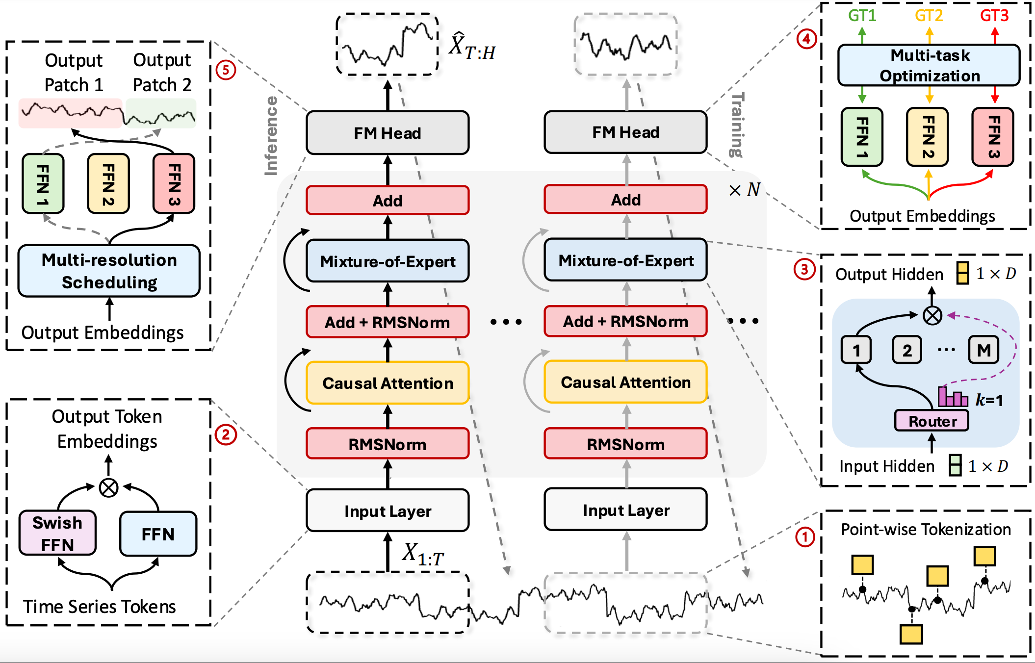
In the first article on the Time-MoE framework, we walked through, step by step, how to turn the abstract ideas from the original paper "Time-MoE: Billion-Scale Time Series Foundation Models with Mixture of Experts" into working MQL5 code. We created the CNeuronSwiGLUOCL module, which transforms raw data into hidden vectors by mixing two projections.
In the second part, we focused on the sparse Mixture of Experts mechanism and implemented it as a single module, CNeuronTimeMoESparseExperts, in which we combined individual and shared data-processing paths, a Top-K router, and a sigmoid gate for the shared expert.
Now it is time to combine all these elements into a complete model and set up its training. Finally, we will test the trained model on real historical data.
Attention Module
Before we begin building the complete model architecture, we need to make one small but extremely important adjustment: replace the standard FeedForward block in the Transformer architecture with the sparse Mixture of Experts module we created. As a reminder, Time-MoE is based on a Decoder-Only architecture in which cross-attention plays a key role, allowing the decoder to take information from the context layer into account.
To do this, we select the ready-made cross-attention component CNeuronCrossDMHAttention as the base class; it provides all the necessary mechanisms. Our task is simply to replace the FeedForward block with a call to CNeuronTimeMoESparseExperts. The structure of the new CNeuronTimeMoEAttention object is shown below.
class CNeuronTimeMoEAttention   :  public CNeuronCrossDMHAttention
  {
protected:
   //---
   virtual bool      feedForward(CNeuronBaseOCL *NeuronOCL) override;
   virtual bool      feedForward(CNeuronBaseOCL *NeuronOCL, CBufferFloat *SecondInput) override
                            { return        feedForward(NeuronOCL); }
   virtual bool      calcInputGradients(CNeuronBaseOCL *prevLayer) override;
   virtual bool      calcInputGradients(CNeuronBaseOCL *NeuronOCL, CBufferFloat *SecondInput,
                     CBufferFloat *SecondGradient, ENUM_ACTIVATION SecondActivation = None) override
                            { return        calcInputGradients(NeuronOCL); }
   virtual bool      updateInputWeights(CNeuronBaseOCL *NeuronOCL) override;
   virtual bool      updateInputWeights(CNeuronBaseOCL *NeuronOCL, CBufferFloat *SecondInput) override
                            { return        updateInputWeights(NeuronOCL); }

public:
                     CNeuronTimeMoEAttention(void)  {};
                    ~CNeuronTimeMoEAttention(void)  {};
   //---
   virtual bool      Init(uint numOutputs, uint myIndex, COpenCLMy *open_cl,
                          uint window, uint window_key, uint units_count,
                          uint window_cross, uint units_cross,
                          uint heads, uint layers,
                          uint experts, uint experts_dimension, uint topK,
                          ENUM_OPTIMIZATION optimization_type, uint batch);
   //---
   virtual int       Type(void) override   const   {  return defNeuronTimeMoEAttention; }
  };
It is worth noting that the CNeuronCrossDMHAttention object is built on the principle of a dynamic internal architecture. This means that the module's key components are not hard-coded in the class structure, but are created on the fly in the required quantity during initialization. The class structure contains only a dynamic array for storing pointers to these objects, which makes it possible to literally reshape the internal layout as needed without modifying the entire codebase: it is enough to adjust the logic in the Init method.
The remaining methods are simply inherited from the parent class or require only minor changes. This approach provides maximum flexibility and reusability, making it easy to create new variations of the module simply by changing the initialization parameters. That is precisely why we focus all our attention on the initialization method — this is where the internal structure of our attention module is born, with the MoE block included.
bool CNeuronTimeMoEAttention::Init(uint numOutputs, uint myIndex, COpenCLMy *open_cl,
                                   uint window, uint window_key, uint units_count,
                                   uint window_cross, uint units_cross, uint heads,
                                   uint layers, uint experts, uint experts_dimension,
                                   uint topK, ENUM_OPTIMIZATION optimization_type, uint batch)
  {
   if(!CNeuronBaseOCL::Init(numOutputs, myIndex, open_cl, window * units_count,
                                                     optimization_type, batch))
      return false;
In the method body, we first call the base neural layer's method of the same name. This allows us to create the module's skeleton. And this is where things get interesting. We prepare the internal layer array cLayers and bind it to our OpenCL interface.
cLayers.Clear();
cLayers.SetOpenCL(OpenCL);
CNeuronRelativeSelfAttention *attention = NULL;
CNeuronRelativeCrossAttention *cross = NULL;
CNeuronTimeMoESparseExperts *MoE = NULL;
bool use_self = units_count > 0;
int layer = 0;
And right away, we set up the necessary local variables. This concludes the preparatory phase.
Then, in a loop over the specified number of internal layers (layers), we gradually build up a single chain. If there is more than one token in the main information stream, we first create and initialize the Self-Attention module, adding it to cLayers. This lets the decoder attend to the tokens it has already generated before switching to external sources of context.
for(uint i = 0; i < layers; i++)
  {
   if(use_self)
     {
      attention = new CNeuronRelativeSelfAttention();
      if(!attention ||
         !attention.Init(0, layer, OpenCL, window, window_key, units_count, heads,
                                                          optimization, iBatch) ||
         !cLayers.Add(attention)
        )
        {
         delete attention;
         return false;
        }
      layer++;
     }
Next, we simply create a cross-attention module that combines information from the previous layer with the context. We pass it the window parameters and the number of attention heads on the fly. It comes online immediately, ready to compute queries, keys, and values. Inside the loop, a pointer to each of these objects is stored in the layer array, as if we were assembling a single processing chain from individual links.
cross = new CNeuronRelativeCrossAttention();
if(!cross ||
   !cross.Init(0, layer, OpenCL, window, window_key, units_count, heads,
                     window_cross, units_cross, optimization, iBatch) ||
   !cLayers.Add(cross)
  )
  {
   delete cross;
   return false;
  }
layer++;
But the main highlight comes right after Cross-Attention: we create an instance of CNeuronTimeMoESparseExperts. This is where we configure our MoE block: we specify the number of experts, the size of their projections (that is, how many features each expert processes), and the topK parameter, which determines how many experts are activated in each pass. And, of course, let's not forget about the connection to the OpenCL context.
 MoE = new CNeuronTimeMoESparseExperts();
 if(!MoE ||
    !MoE.Init(0, layer, OpenCL, window, experts_dimension, units_count, 1,
                                   experts, topK, optimization, iBatch) ||
    !cLayers.Add(MoE)
   )
   {
    delete MoE;
    return false;
   }
 layer++;
}
Once the initialization loop for all layers is complete, we connect the result buffers of the last layer to the object's external interfaces.
   SetOutput(MoE.getOutput(), true);
   SetGradient(MoE.getGradient(), true);
//---
   return true;
  }
As a result, the Init method transforms an empty container into a living organism consisting of three types of layers arranged in a strict sequence, and it does so without making a single modification to the underlying attention mechanisms. All the dynamics are created solely by adding new elements and configuring them parametrically — a classic example of a flexible architecture that requires minimal maintenance.
But there is one catch. The cross-attention module requires two information streams: the main stream and the context stream. But in the Time-MoE framework, there is only one. This issue is addressed with minimal intervention in the core mechanisms. We simply override the forward and backward pass methods, which take a single information stream as input and route it in two directions.
bool CNeuronTimeMoEAttention::feedForward(CNeuronBaseOCL *NeuronOCL)
  {
   if(!NeuronOCL)
      return false;
   return CNeuronCrossDMHAttention::feedForward(NeuronOCL, NeuronOCL.getOutput());
  }
At first glance, this operation turns the Cross-Attention module into a Self-Attention module. But our idea is to pass only the tokens from the most recent time step through the main information stream. This is achieved by reducing the number of elements analyzed in the main information stream. Through the context information stream, we pass the complete set of information, allowing the tokens in the main information stream to be enriched with the entire historical context. Thanks to this, all the advantages of the Decoder-Only Time-MoE architecture are preserved: each new token seeks advice from the experts about its narrow subspace while simultaneously relying on all the accumulated market dynamics.
The complete code for this class and all of its methods is provided in the attachment.
Model Architecture
Now that all the necessary components have been implemented, we finally move on to building the full architecture of the trainable models. As in previous works, the project remains based on the Actor–Director–Critic framework, which has proven effective in reinforcement learning tasks. It is within this framework that we integrate all our developments related to Time-MoE, incorporating them into the Environment State Encoder — the part of the model responsible for generating a semantically rich representation of the input data.
However, an important point arises at this stage. The overall pipeline we use has only a single model output — a universal feature vector used by all components: Actor, Director, and Critic. At the same time, the authors' Time-MoE architecture includes several forecasting heads, each working with a different planning horizon. This creates a potential conflict. Combining all outputs into a single buffer makes training more complicated and reduces interpretability.
We decided not to combine everything into a single structure. Instead, a clear logical separation was implemented between the Encoder and the forecasting heads. The encoder (Time-MoE) acts as a universal feature extraction mechanism — it is a single shared component for all of them. Next, for each planning horizon, a separate model is created that receives the outputs of the Encoder as input and generates a forecast for its own task.
This approach offers tangible benefits: we retain a single trainable unit for extracting information, while at the same time ensuring independence and flexibility at the forecasting level. Each head is responsible for its own time scale, which means it can adapt to the corresponding nature of market fluctuations. As a result, the architecture remains modular and scalable, while at the same time being highly adaptable to the structure of the temporal context.
After establishing the overall logic of the framework, we move on to designing the architecture of the trainable models, in which each subsystem is built according to a common principle. This ensures structural clarity and allows the model to be scaled flexibly to meet the needs of the trading core.
All initialization is handled in the CreateDescriptions method, which assembles the architectures layer by layer, starting with the Encoder.
bool CreateDescriptions(CArrayObj *&encoder,
                        CArrayObj *&forecast1,
                        CArrayObj *&forecast2,
                        CArrayObj *&forecast3,
                        CArrayObj *&actor,
                        CArrayObj *&director,
                        CArrayObj *&critic
                       )
  {
//---
   CLayerDescription *descr;
//---
   if(!encoder)
     {
      encoder = new CArrayObj();
      if(!encoder)
         return false;
     }
   if(!forecast1)
     {
      forecast1 = new CArrayObj();
      if(!forecast1)
         return false;
     }
   if(!forecast2)
     {
      forecast2 = new CArrayObj();
      if(!forecast2)
         return false;
     }
   if(!forecast3)
     {
      forecast3 = new CArrayObj();
      if(!forecast3)
         return false;
     }
   if(!actor)
     {
      actor = new CArrayObj();
      if(!actor)
         return false;
     }
   if(!director)
     {
      director = new CArrayObj();
      if(!director)
         return false;
     }
   if(!critic)
     {
      critic = new CArrayObj();
      if(!critic)
         return false;
     }
Raw historical market data is fed into the Encoder. The first layer is simply a base object that essentially serves as an interface for retrieving data. Next comes a batch normalization layer with added noise, which stabilizes the distribution of the input values, provides some data augmentation, and helps prevent the model from overfitting.
//--- Encoder
   encoder.Clear();
//--- Input layer
   if(!(descr = new CLayerDescription()))
      return false;
   descr.type = defNeuronBaseOCL;
   uint prev_count = descr.count = (HistoryBars * BarDescr);
   descr.activation = None;
   descr.optimization = ADAM;
   if(!encoder.Add(descr))
     {
      delete descr;
      return false;
     }
//--- layer 1
   if(!(descr = new CLayerDescription()))
      return false;
   descr.type = defNeuronBatchNormWithNoise;
   descr.count = prev_count;
   descr.batch = BatchSize;
   descr.activation = None;
   descr.optimization = ADAM;
   if(!encoder.Add(descr))
     {
      delete descr;
      return false;
     }
Next, a ConcatDiff layer is used, which adds channels of differential values by breaking each bar down into its components and preparing the data structure for more complex processing.
//--- layer 2
   if(!(descr = new CLayerDescription()))
      return false;
   descr.type = defNeuronConcatDiff;
   prev_count = descr.count = HistoryBars;
   descr.layers = BarDescr;
   descr.step = 1;
   descr.batch = BatchSize;
   descr.optimization = ADAM;
   descr.activation = None;
   if(!encoder.Add(descr))
     {
      delete descr;
      return false;
     }
After that, the data enters the Mamba4CastEmbedding module. It is here that the input sequence is enriched with tags from multiple time scales simultaneously. This mechanism makes it possible to obtain a multi-frequency representation of the input signal. This layer outputs a fixed-length latent window (NSkills), which then passes through a transposition layer that changes the tensor dimensions into a form suitable for subsequent processing of independent univariate sequences of individual channels.
//--- layer 3
   if(!(descr = new CLayerDescription()))
      return false;
   descr.type = defMamba4CastEmbeding;
   prev_count = descr.count = HistoryBars;
   descr.window = 2 * BarDescr;
   uint prev_out = descr.window_out = NSkills;
     {
      uint temp[] = {PeriodSeconds(PERIOD_H1), PeriodSeconds(PERIOD_D1)};
      if(ArrayCopy(descr.windows, temp) < (int)temp.Size())
         return false;
     }
   descr.batch = BatchSize;
   descr.optimization = ADAM;
   descr.activation = None;
   if(!encoder.Add(descr))
     {
      delete descr;
      return false;
     }
//--- layer 4
   if(!(descr = new CLayerDescription()))
      return false;
   descr.type = defNeuronTransposeOCL;
   descr.count = prev_count;
   prev_count = descr.window = prev_out;
   descr.batch = BatchSize;
   descr.optimization = ADAM;
   descr.activation = None;
   if(!encoder.Add(descr))
     {
      delete descr;
      return false;
     }
   prev_out = descr.count;
Next comes a SwiGLU embedding layer. It increases the feature depth and forms the initial basis for an abstract representation of the state.
//--- layer 5
   if(!(descr = new CLayerDescription()))
      return false;
   descr.type = defNeuronSwiGLUOCL;
   descr.count = Segments;
   descr.window = (prev_out + Segments - 1) / Segments;
   descr.variables = prev_count;
   prev_out = descr.window_out = EmbeddingSize;
   descr.batch = BatchSize;
   descr.optimization = ADAM;
   descr.activation = None;
   if(!encoder.Add(descr))
     {
      delete descr;
      return false;
     }
   prev_count = descr.count;
   uint prev_var = descr.variables;
Next, the TransposeRCDOCL transposition layer is applied, allowing the dimensions of the time steps and the analyzed channels to be rearranged. This operation is critical for the correct operation of the attention module we have created. It is precisely thanks to this operation that tokens from the most recent time step for all analyzed variables are collected at the beginning of the buffer.
//--- layer 6
   if(!(descr = new CLayerDescription()))
      return false;
   descr.type = defNeuronTransposeRCDOCL;
   descr.count = prev_var;
   descr.window = prev_count;
   descr.step = prev_out;
   descr.batch = BatchSize;
   descr.optimization = ADAM;
   descr.activation = None;
   if(!encoder.Add(descr))
     {
      delete descr;
      return false;
     }
//--- layer 7
   if(!(descr = new CLayerDescription()))
      return false;
   descr.type = defNeuronBatchNormOCL;
   descr.count = prev_count * prev_out * prev_var;
   descr.batch = BatchSize;
   descr.activation = None;
   descr.optimization = ADAM;
   if(!encoder.Add(descr))
     {
      delete descr;
      return false;
     }
This is followed by a batch normalization layer, which stabilizes the data distribution before it is passed to the attention module.
And now we have reached the key module — TimeMoEAttention. This is a multi-head attention module with numerous experts, each of which focuses on its own aspect of temporal information. As input, it receives compact tokens representing the current state and context drawn from the entire history — in this way, the tokens extract the meaning out of the data. The input dimensions and the number of experts (NExperts) are specified via parameters, and each head selects the Top-K experts, forming a compact yet expressive latent representation. This layer is the final one in the encoder and defines the output space that all forecasting and decision-making models will subsequently access.
//--- layer 8
   if(!(descr = new CLayerDescription()))
      return false;
   descr.type = defNeuronTimeMoEAttention;
   descr.window_out = EmbeddingSize / 4;
     {
      uint temp[] = {prev_out, prev_out, 8, TopK};               //Window Main, Window Cross, Experts dimension, TopK
      if(ArrayCopy(descr.windows, temp) < ArraySize(temp))
         return false;
     }
     {
      uint temp[] = {prev_var, prev_var * prev_count, NExperts}; //Units Main, Units Cross, Experts
      if(ArrayCopy(descr.units, temp) < ArraySize(temp))
         return false;
     }
   descr.layers = 6;
   descr.step = 4;                                                // Attention heads
   descr.batch = BatchSize;
   descr.activation = None;
   descr.optimization = ADAM;
   if(!encoder.Add(descr))
     {
      delete descr;
      return false;
     }
At the encoder output, a shared latent array is formed and made accessible to all models. The first forecasting model, forecast1, takes it as is. The base input layer receives the tensor. This is followed by simple convolutional processing, which generates a forecast for the specified planning horizon for each channel under analysis. In this case, only the next value is forecast.
//---
   CLayerDescription *latent = descr;
//--- Forecast 1
   forecast1.Clear();
//--- Input layer
   if(!(descr = new CLayerDescription()))
      return false;
   descr.type = defNeuronBaseOCL;
   descr.count = int(latent.windows[0] * latent.units[0]);
   descr.activation = None;
   descr.optimization = ADAM;
   if(!forecast1.Add(descr))
     {
      delete descr;
      return false;
     }
//--- layer 1
   if(!(descr = new CLayerDescription()))
      return false;
   descr.type = defNeuronConvOCL;
   descr.count = latent.units[0];
   descr.window = latent.windows[0];
   descr.step = descr.window;
   descr.layers = 1;
   descr.window_out = 1;
   descr.batch = BatchSize;
   descr.optimization = ADAM;
   descr.activation = TANH;
   if(!forecast1.Add(descr))
     {
      delete descr;
      return false;
     }
Here, it is worth paying special attention to one important technical detail. During the data preprocessing performed by the Environment State Encoder, the original feature space was intentionally expanded. This expansion is necessary for extracting high-level features and forming a more expressive latent representation. However, this transformation results in a dimensionality mismatch between the predicted values and the actual data we use during the training phase.
To ensure that the forecast results are correctly aligned with the true values, the forecasts must be mapped back to the scale and structure of the original space. In this case, this is achieved by using a simple fully connected layer that reduces the data dimensionality to the specified value BarDescr.
//--- layer 2
   if(!(descr = new CLayerDescription()))
      return false;
   descr.type = defNeuronBaseOCL;
   descr.count = BarDescr;
   descr.activation = TANH;
   descr.optimization = ADAM;
   if(!forecast1.Add(descr))
     {
      delete descr;
      return false;
     }
The second point worth addressing separately is the restoration of the original data distribution that was lost during normalization. Previously, we used the RevIN inverse normalization layer for this purpose, which automatically extracts the normalization parameters from the corresponding layer in the Encoder. However, an architectural limitation has arisen in the current implementation: the normalization layer remains inside the Environment Encoder and is not directly accessible from the forecasting models. In other words, RevIN simply will not work here — there is no access to the batch statistics.
At first glance, the solution may seem paradoxical: we use a batch normalization layer again — but not for normalization, rather for restoring the original scale. Yes, yes, it sounds like a pun, but in practice, it is a perfectly valid technique.
The point is that the BatchNorm architecture has two output parameters: scaling (scale) and offset (bias), which can be trainable. Although they are traditionally used to stabilize and accelerate training, in our case they take on a different role — learning the inverse transformation that brings the forecast values closer to the original distribution. Thus, instead of storing normalization statistics, we allow the model itself to learn how to denormalize the data, adapting to real-world conditions.
This approach has a certain elegance: it keeps the model structure compact, avoids unnecessarily complicating the state buffer, and, importantly, does not break the computational graph, ensuring full compatibility with the current backpropagation logic.
//--- layer 3
   if(!(descr = new CLayerDescription()))
      return false;
   descr.type = defNeuronBatchNorm;
   descr.count = BarDescr;
   descr.batch = BatchSize;
   descr.activation = None;
   descr.optimization = ADAM;
   if(!forecast1.Add(descr))
     {
      delete descr;
      return false;
     }
Everything is designed for maximum efficiency: a constant window, a single layer, and a fixed length.
The second and third forecasting models (forecast2, forecast3) use the same input data as the first. They almost completely replicate its architecture, but differ in having a longer forecast window. The parameters of the forecasting convolutional layer are copied from the first head, but the number of filters is expanded to the required planning horizon.
//--- Forecast 2
   forecast2.Clear();
//--- Input layer
   if(!forecast2.Add(forecast1.At(0)))
      return false;
//--- layer 1
   if(!(descr = new CLayerDescription()))
      return false;
   if(!descr.Copy(forecast1.At(1)))
     {
      delete descr;
      return false;
     }
   prev_out = descr.window_out = NForecast / 2;
   if(!forecast2.Add(descr))
     {
      delete descr;
      return false;
     }
   prev_count = descr.count;
Another technically important point concerns the architecture of the forecasting block. At the output of the convolutional layer, the model generates forecast values for individual univariate time series, each of which reflects the local dynamics of a specific indicator or feature. This makes the forecast structure spatially sparse but information-rich.
This raises the question: how can these forecasts be aggregated and converted into a form comparable to the source data? In principle, one could use a classic fully connected layer — it is quite capable of aggregating information. However, as the planning horizon increases (and, consequently, the length of the output sequence), this implementation becomes less efficient. The number of parameters grows explosively, and local temporal dependencies begin to be lost.
To avoid this, we first transpose the tensor, rearranging the axes so that the time steps become independent channels. This allows the next convolutional layer to be applied to each time slice separately. In other words, instead of processing the entire sequence as a single whole, we allow the model to analyze each point in time through the lens of its own features. This operation offers a twofold benefit: it reduces the dimensionality of the output representation (thereby acting as a bottleneck) while simultaneously preserving temporal coherence between steps.
//--- layer 2
   if(!(descr = new CLayerDescription()))
      return false;
   descr.type = defNeuronTransposeOCL;
   descr.window = prev_out;
   descr.count = prev_count;
   descr.batch = BatchSize;
   descr.optimization = ADAM;
   descr.activation = None;
   if(!forecast2.Add(descr))
     {
      delete descr;
      return false;
     }
//--- layer 3
   if(!(descr = new CLayerDescription()))
      return false;
   descr.type = defNeuronConvOCL;
   descr.window = prev_count;
   descr.step = prev_count;
   prev_count = descr.count = prev_out;
   descr.layers = 1;
   prev_out = descr.window_out = BarDescr;
   descr.batch = BatchSize;
   descr.optimization = ADAM;
   descr.activation = TANH;
   if(!forecast2.Add(descr))
     {
      delete descr;
      return false;
     }
Thus, an effective aggregation mechanism is implemented without losing the detailed structure of the forecast. This is especially valuable when training models on data with high multiplicity and when using multi-graph features, where each time slice carries specific information that cannot be reduced to a general pattern.
The process concludes with a final batch normalization step that restores the original data distribution.
//--- layer 4
   if(!(descr = new CLayerDescription()))
      return false;
   descr.type = defNeuronBatchNormOCL;
   descr.count = prev_count * prev_out;
   descr.activation = None;
   if(!forecast2.Add(descr))
     {
      delete descr;
      return false;
     }
The model functions as a longer-horizon forecasting model, using the same features but interpreting them through a higher-magnification lens.
As for the third forecasting model, its architecture is identical to that of the second one. The only difference is the extended planning horizon, which allows us to look further into the future. Otherwise, it uses the same convolutional and transposed layers, as well as the same logic for dimensionality matching and normalization. Therefore, to avoid cluttering the discussion with repetition, we will omit its detailed description and focus on decision-making models.
Next comes the Actor model, that is, the strategy executor. It receives descriptors of the current account state as input. The resulting data undergo standard normalization.
//--- Actor
   actor.Clear();
//--- Input layer
   if(!(descr = new CLayerDescription()))
      return false;
   descr.type = defNeuronBaseOCL;
   descr.count = AccountDescr;
   descr.activation = None;
   descr.optimization = ADAM;
   if(!actor.Add(descr))
     {
      delete descr;
      return false;
     }
//--- layer 1
   if(!(descr = new CLayerDescription()))
      return false;
   descr.type = defNeuronBatchNormOCL;
   descr.count = AccountDescr;
   descr.batch = BatchSize;
   descr.activation = None;
   descr.optimization = ADAM;
   if(!actor.Add(descr))
     {
      delete descr;
      return false;
     }
They are then fed into the CrossDMHAttention mechanism. This is a cross-attention mechanism where the main stream consists of current account information, and the context consists of latent features from the Encoder. This approach allows the model's attention mechanism to identify the most relevant features from the market state, taking into account the user's current situation. Inside the block, there is a stack of three attention layers, each of which uses several attention heads.
//--- layer 2
   if(!(descr = new CLayerDescription()))
      return false;
   descr.type = defNeuronCrossDMHAttention;
     {
      uint temp[] = {AccountDescr,         // Inputs window
                    latent.windows[0]     // Cross window
                   };
      if(ArrayCopy(descr.windows, temp) < (int)temp.Size())
         return false;
     }
     {
      uint temp[] = {1,                 // Inputs units
                    latent.units[0]    // Cross units
                   };
      if(ArrayCopy(descr.units, temp) < (int)temp.Size())
         return false;
     }
   descr.step = 4;                  // Heads
   descr.window_out = 32;
   descr.batch = 1e4;
   descr.layers = 3;
   descr.activation = None;
   descr.optimization = ADAM;
   if(!actor.Add(descr))
     {
      delete descr;
      return false;
     }
After the attention mechanism comes a chain of three fully connected layers, which transforms the resulting data into action probabilities (NActions). It is this output that is used when generating trading decisions.
//--- layer 3
   if(!(descr = new CLayerDescription()))
      return false;
   descr.type = defNeuronBaseOCL;
   descr.count = LatentCount;
   descr.batch = BatchSize;
   descr.activation = TANH;
   descr.optimization = ADAM;
   if(!actor.Add(descr))
     {
      delete descr;
      return false;
     }
//--- layer 4
   if(!(descr = new CLayerDescription()))
      return false;
   descr.type = defNeuronBaseOCL;
   descr.count = LatentCount;
   descr.activation = SoftPlus;
   descr.batch = BatchSize;
   descr.optimization = ADAM;
   if(!actor.Add(descr))
     {
      delete descr;
      return false;
     }
//--- layer 5
   if(!(descr = new CLayerDescription()))
      return false;
   descr.type = defNeuronBaseOCL;
   prev_count = descr.count = NActions;
   descr.activation = SIGMOID;
   descr.batch = BatchSize;
   descr.optimization = ADAM;
   if(!actor.Add(descr))
     {
      delete descr;
      return false;
     }
Thus, the entire architecture is structured sequentially, logically, and modularly: from preprocessing historical data, through transformer mechanisms and multi-head attention, to forecasting and decision-making. This approach ensures transparency, reliability, and sufficient flexibility — which is especially important for real-world trading applications, where the architecture does not tolerate fragmentation. Everything is anchored to a common latent space, and each model operates within its own context without losing global consistency.
The Critic and Director model architectures are structured similarly to the Actor model. The only difference is that the input is not the account state, but an action vector generated by the Actor itself. The output is a numerical evaluation of these actions: for the Critic, this is the value function, while for the Director, it is a signal gradient from binary classification (good/bad action). The internal structure consists of the same normalization blocks, the cross-attention mechanism, and a cascade of output layers. To avoid cluttering the text with repetitions of details already covered, we will not dwell on them in detail. The complete architecture of all components is provided in the attachment.
Model Training
The next step in our work is training the models. This is where one of the key challenges awaits us. The authors of the original Time-MoE framework trained their neural networks on the massive, if not colossal, Time-300B dataset. This dataset covers more than 300 billion time points from nine different domains, including economics, energy, transportation, healthcare, and others. This volume of data gives the model impressive generalization capability — but it also requires resources that are not available in a local or semi-automated training setup.
It would be unrealistic to replicate such a dataset at home. However, limiting ourselves to online training on incoming data alone means creating a system that is inherently incapable of learning stable patterns. This is especially true under conditions of high market volatility and a limited observation window.
Therefore, we adopted a compromise solution: to abandon the preliminary stage of collecting a static training dataset, while maintaining control over the training process through the step-by-step accumulation and use of internal state buffers. Here, we relied on a mechanism previously tested in the TimeFound model — it proved effective enough to be reused, but this time not only for training the forecasting model, but also for training decision-making models.
The mechanism essentially consists of training the agent on pseudo-real data. Here, the actual quote history is obtained from the trading terminal, while actions are evaluated by a simulated environment. The entire process is built within the Train method of the "…\Experts\TimeMoE\Study.mq5" Expert Advisor. This is where the step-by-step processing of historical data begins, along with the formation of training batches, the collection of trading account context, and the sequential training of the model using backpropagation.
In the first stage, the method determines the training time boundaries: the start and end indices of the historical interval on which training will be performed are calculated.
void Train(void)
  {
   int start = iBarShift(Symb.Name(), TimeFrame, Start);
   int end = iBarShift(Symb.Name(), TimeFrame, End);
   int bars = CopyRates(Symb.Name(), TimeFrame, 0, start, Rates);
Next, the price quotes are loaded and the main technical indicators are initialized. Each of them is checked for readiness — if the calculations have not yet been completed, the system waits, inserting short pauses. This is necessary for stable buffer initialization; otherwise, subsequent processing simply would not be meaningful.
   if(!RSI.BufferResize(bars) || !CCI.BufferResize(bars) ||
      !ATR.BufferResize(bars) || !MACD.BufferResize(bars))
     {
      PrintFormat("%s -> %d", __FUNCTION__, __LINE__);
      ExpertRemove();
      return;
     }
//---
   int count = -1;
   bool calculated = false;
   do
     {
      count++;
      calculated = (RSI.BarsCalculated() >= bars &&
                    CCI.BarsCalculated() >= bars &&
                    ATR.BarsCalculated() >= bars &&
                    MACD.BarsCalculated() >= bars
                   );
      Sleep(100);
      count++;
     }
   while(!calculated && count < 100);
   if(!calculated)
     {
      PrintFormat("%s -> %d The training data has not been loaded", __FUNCTION__, __LINE__);
      ExpertRemove();
      return;
     }
   RSI.Refresh();
   CCI.Refresh();
   ATR.Refresh();
   MACD.Refresh();
//---
   if(!ArraySetAsSeries(Rates, true))
     {
      PrintFormat("%s -> %d", __FUNCTION__, __LINE__);
      ExpertRemove();
      return;
     }
   bars -= end + HistoryBars + NForecast;
   if(bars < 0)
     {
      PrintFormat("%s -> %d", __FUNCTION__, __LINE__);
      ExpertRemove();
      return;
     }
As soon as the indicators are ready, the process of collecting patterns for training begins. We set up a training loop in which, at each iteration, a random position within the valid range of bars is selected. This is the entry point for the next training scenario. Based on this position, three key vectors are formed:
- bState — describes the market state as a tensor of indicators and price parameters;
- bTime — reflects the temporal context;
- Result — contains a target forecast based on future price behavior.
   vector<float> result, target, neg_target;
   bool Stop = false;
//---
   uint ticks = GetTickCount();
//---
   for(int iter = 0; (iter < Iterations && !IsStopped() && !Stop); iter ++)
     {
      int posit = (int)((MathRand() * MathRand() / MathPow(32767, 2)) * bars);
      if(!CreateBuffers(posit + end, GetPointer(bState), GetPointer(bTime), Result))
        {
         PrintFormat("%s -> %d", __FUNCTION__, __LINE__);
         ExpertRemove();
         return;
        }
In addition to the market state, a pseudo-account state is generated — a simulation of the trader’s trading context at this stage. This occurs in the SampleAccount function, which creates a feature vector that includes balance, equity, position size, accumulated profit, the risk-to-take-profit and risk-to-stop-loss ratios, as well as sinusoidal signals that model hidden seasonal patterns.
const vector<float> account = SampleAccount(GetPointer(bState), datetime(bTime[0]));
if(!bAccount.AssignArray(account))
  {
   PrintFormat("%s -> %d", __FUNCTION__, __LINE__);
   ExpertRemove();
   return;
  }
This vector is fed as input to the actor, broadening its understanding of the current situation: the agent makes decisions not only based on the market, but also in the context of its trading position.
Once the input data has been prepared, the model performs its forward pass: the Encoder encodes the market, after which three Forecast[i] blocks generate forecasts for different time horizons.
//--- Feed Forward
if(!cEncoder.feedForward((CBufferFloat*)GetPointer(bState), 1, false, (CBufferFloat*)GetPointer(bTime)))
  {
   PrintFormat("%s -> %d", __FUNCTION__, __LINE__);
   Stop = true;
   break;
  }
for(uint f = 0; f < caForecast.Size(); f++)
   if(!caForecast[f].feedForward(GetPointer(cEncoder), -1, (CBufferFloat*)NULL))
     {
      PrintFormat("%s -> %d - Forecast %d", __FUNCTION__, __LINE__, f);
      Stop = true;
      break;
     }
At the same time, the Actor generates a trading decision, which is immediately evaluated by two independent models — the Critic and the Director. One analyzes the decision from the perspective of the classic value-based approach, while the other treats it as a binary classifier that provides strong feedback, distinguishing good actions from clearly erroneous ones.
if(!cActor.feedForward(GetPointer(bAccount), 1, false, GetPointer(cEncoder), LatentLayer))
  {
   PrintFormat("%s -> %d", __FUNCTION__, __LINE__);
   Stop = true;
   break;
  }
if(!cCritic.feedForward(GetPointer(cActor), -1, GetPointer(cEncoder), LatentLayer))
  {
   PrintFormat("%s -> %d", __FUNCTION__, __LINE__);
   Stop = true;
   break;
  }
if(!cDirector.feedForward(GetPointer(cActor), -1, GetPointer(cEncoder), LatentLayer))
  {
   PrintFormat("%s -> %d", __FUNCTION__, __LINE__);
   Stop = true;
   break;
  }
Next, we move on to optimizing the model parameters by calling the backward pass method. A tensor of subsequent environment states prepared in advance is used to train the forecasting models.
//--- Study
for(uint f = 0; f < caForecast.Size(); f++)
   if(!caForecast[f].backProp(Result, (CBufferFloat*)NULL) ||
      !cEncoder.backPropGradient((CBufferFloat*)NULL))
     {
      PrintFormat("%s -> %d - Forecast %d", __FUNCTION__, __LINE__, f);
      Stop = true;
      break;
     }
The CheckAction function is used to obtain an objective assessment of an action. It simulates the opening of a virtual position and calculates the expected profit, taking into account a discount factor based on actual historical data. Based on these data, a reward is generated, which is fed back into the model and serves as the basis for recalculating the parameters of all components — the Actor, Critic, and Director.
cActor.getResults(Action);
double equity = bAccount[2] * bAccount[0] * EtalonBalance / (1 + bAccount[1]);
double reward = CheckAction(Action, Result, equity);
Result.Clear();
if(!Result.Add(float(reward)))
  {
   PrintFormat("%s -> %d", __FUNCTION__, __LINE__);
   Stop = true;
   break;
  }
if(!cCritic.backProp(Result, GetPointer(cEncoder), LatentLayer) ||
   !cActor.backPropGradient(GetPointer(cEncoder), LatentLayer, -1, true))
  {
   PrintFormat("%s -> %d", __FUNCTION__, __LINE__);
   Stop = true;
   break;
  }
if(!Result.Update(0, float(reward > 0)))
  {
   PrintFormat("%s -> %d", __FUNCTION__, __LINE__);
   Stop = true;
   break;
  }
if(!cDirector.backProp(Result, GetPointer(cEncoder), LatentLayer) ||
   !cActor.backPropGradient(GetPointer(cEncoder), LatentLayer, -1, true))
  {
   PrintFormat("%s -> %d", __FUNCTION__, __LINE__);
   Stop = true;
   break;
  }
Gradient correction occurs quickly, in a single update. The errors are fed back into the network, and the weights are updated according to the training signal. This allows the model to gradually accumulate useful patterns and adjust its behavior based on new examples, learning to avoid mistakes and reinforce useful actions.
To provide real-time visual monitoring of the process, the method periodically displays key training parameters in the chart comments: forecast errors and critic accuracy.
 if(GetTickCount() - ticks > 500)
   {
    double percent = double(iter) * 100.0 / (Iterations);
    string str = "";
    for(uint f = 0; f < caForecast.Size(); f++)
       str += StringFormat("%-12s%d %6.2f%% -> Error %15.8f\n", "Forecast", f, percent,
                                                caForecast[f].getRecentAverageError());
    str += StringFormat("%-12s %6.2f%% -> Error %15.8f\n", "Critic", percent,
                                                      cCritic.getRecentAverageError());
    str += StringFormat("%-12s %6.2f%% -> Error %15.8f\n", "Director", percent,
                                                    cDirector.getRecentAverageError());
    Comment(str);
    ticks = GetTickCount();
   }
}
Upon completion of the specified number of iterations, the method outputs the training results to the terminal log and cleanly terminates the program using ExpertRemove.
   Comment("");
//---
   for(uint f = 0; f < caForecast.Size(); f++)
      PrintFormat("%s -> %d -> %-15s%d %10.7f", __FUNCTION__, __LINE__, "Forecast", f,
                                               caForecast[f].getRecentAverageError());
   PrintFormat("%s -> %d -> %-15s %10.7f", __FUNCTION__, __LINE__, "Critic",
                                                     cCritic.getRecentAverageError());
   PrintFormat("%s -> %d -> %-15s %10.7f", __FUNCTION__, __LINE__, "Director",
                                                   cDirector.getRecentAverageError());
   ExpertRemove();
//---
  }
Thus, each training run is a series of small simulations, each of which recreates a segment of history: from the market state to the trading result. The agent learns through direct experience, through mistakes and successful actions, gradually adapting to various market conditions and improving its own strategy through a balanced evaluation system and targeted correction.
After the main training phase, the model moves on to fine-tuning, which is performed in online learning mode. For this, the built-in MetaTrader 5 Strategy Tester is used, allowing the algorithm to be run under conditions that are as close as possible to the real market while keeping the simulation fully controllable. This approach makes it possible not only to assess the model's quality, but also to adapt its behavior to the current market environment, gradually tuning its parameters to current volatility and the nature of price movement.
The online learning mechanism is implemented based on the program carried over from previous works, without any changes. The model continues to learn from new data, adjusting its actions on the fly, which is particularly important when market regimes change frequently.
Testing
The model training process was divided into two stages. This approach made it possible to build the system in a consistent, reliable, and unhurried way.
First comes offline training. We used 15 years of history for the EURUSD pair on the M1 timeframe. This provided the model with a large volume of diverse market situations. The Encoder learned to recognize regularities, identify significant patterns, and encode the market state into a compact, information-rich feature vector. This vector serves as the foundation for all decisions made by the agent. During training, the Actor learns a behavioral strategy by receiving signals from the Critic and the Director.
Then comes online fine-tuning. It is run in the MetaTrader 5 Strategy Tester. Here, the model interacts with historical data in a realistic mode: candlestick by candlestick, with market noise, random fluctuations, and instability. This helps adapt the agent's behavior to live market dynamics and adjust its strategy under near-real conditions.
After training, the model was tested on new data — quotes for January 2025. All settings were fixed in advance and remained unchanged. This ensures that the evaluation is objective and transparent. The test results are shown below.
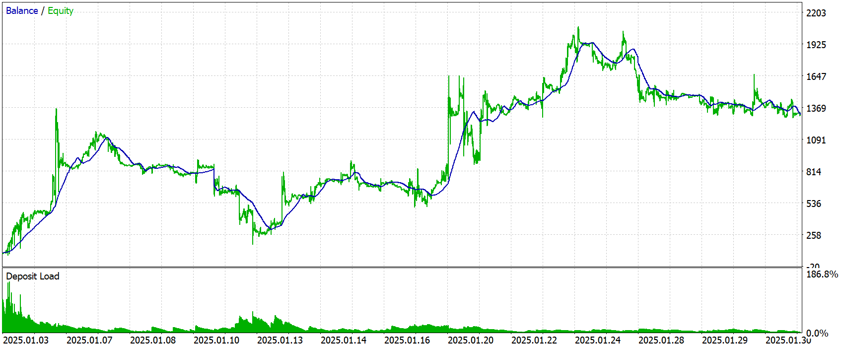
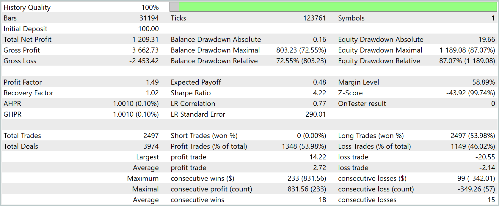
The test results look mixed and should be interpreted with caution. On the one hand, cumulative return is traditionally important: with an initial deposit of $100, the system ended the period with a net profit of $1,209. That is 12 times the initial capital. The balance chart shows steady growth until mid-month, followed by relative stabilization at the $1,350–1,400 level.
However, the extreme drawdown is immediately apparent. The maximum balance drawdown exceeded 72%, while the equity drawdown exceeded 87%. This means that during the most severe periods of trading, the system lost most of its capital. This characterizes the behavior policy as high-risk, even despite the subsequent recovery.
The Profit Factor was 1.49 — many consider this an acceptable level, but with such drawdowns, it is unlikely to compensate for potential losing periods. The Recovery Factor (the ratio of net profit to maximum drawdown) is nearly 1, which indicates a very slow recovery from losses.
Trading statistics show that nearly 2,500 trades were opened during the month, of which 53.98% were profitable. The average profit is only slightly greater than the average loss.
Overall, these results show that the model is capable of identifying profitable signals and generating account growth, but it does so at the cost of very deep drawdowns and long streaks of losing trades. For practical trading, this strategy requires additional protection to reduce the risk of a deep drawdown in capital.
Conclusion
In this work, we took the key ideas of the Time‑MoE framework from the academic paper and translated them into real code in MQL5 and OpenCL, step by step. We implemented the SwiGLU embedding, constructed a sparse Mixture of Experts, and integrated it into the cross-attention mechanism. We set up a complete training pipeline within the Actor–Director–Critic architecture. Thanks to a clear modular structure, all components were interconnected while remaining easy to configure and extend.
The first phase of offline training on fifteen years of data allowed the Encoder to form a rich latent representation of the market, and the Actor to master a basic strategy under the supervision of the Critic and the Director. The second stage of online fine-tuning in the MetaTrader 5 Strategy Tester made the model ready for trading by reflecting the dynamics and noise of the modern market in its parameters.
Testing on January 2025 quotes showed that the Agent is capable of generating steady profits, but is accompanied by deep drawdowns. This points to the need for further optimization of risk management and fine-tuning of trading criteria.
Links
- Time-MoE: Billion-Scale Time Series Foundation Models with Mixture of Experts
- Other articles in this series
Software used in the article
| # | Name | Type | Description |
|---|---|---|---|
| 1 | Study.mq5 | Expert Advisor | Expert Advisor for offline model training |
| 2 | StudyOnline.mq5 | Expert Advisor | Expert Advisor for online model training |
| 3 | Test.mq5 | Expert Advisor | Expert Advisor for model testing |
| 4 | Trajectory.mqh | Class Library | Structure describing the system state and model architecture |
| 5 | NeuroNet.mqh | Class Library | Class library for creating neural networks |
| 6 | NeuroNet.cl | Library | Code library for the OpenCL program |
Translated from Russian by MetaQuotes Ltd.
Original article: https://www.mql5.com/ru/articles/18548
Warning: All rights to these materials are reserved by MetaQuotes Ltd. Copying or reprinting of these materials in whole or in part is prohibited.
This article was written by a user of the site and reflects their personal views. MetaQuotes Ltd is not responsible for the accuracy of the information presented, nor for any consequences resulting from the use of the solutions, strategies or recommendations described.

 Detecting Structural Breakpoints in Price Series Using CUSUM in MQL5 (Part 2): Implementing the Detector as a Native MQL5 Indicator
 Automating Terminal Startup for Service Tasks
 Measuring What Matters (Part 3): The Reconstruction Engine — Validating Risk Footprints with Matrix Algebra
 How to Detect and Normalize Chart Objects in MQL5 (Part 5): Fibonacci in Focus

- Free trading apps
- Over 8,000 signals for copying
- Economic news for exploring financial markets
You agree to website policy and terms of use
Thank you for sharing your codes. It's been a while I'm following your articles. They all look to be written based upon very recent academic publications. But I have issues to compile them as all run into too many syntax errors. Many of the errors are originated from the "NeuroNet.cl", which if I am correct is the core of OpenCl computing for "NeuroNet.mqh". I am confident that all the codes are compiled already on your side. So I assume that the issues come from the MQL version on my side which might be different than yours. Could you give us a little details about it? Thank you!
[T]rades are only on long side[.]
IMHO, a longs-only algo is likely better for something like the S&P 500 Index that has more consistent upward time.
Of course, the EURUSD is merely a demonstration of the concepts and work in the Article so...