Neural Networks in Trading: Adaptive Periodic Segmentation (LightGTS)

Introduction

Time series forecasting has long been a key tool in many fields — from energy and transportation to healthcare and education. But it is precisely in finance — where the value of every second can be measured in monetary terms — that the accuracy of a forecast becomes critically important. There is no room for error here: even the slightest misstep in the model — and the strategy goes into the red.

Traditional approaches, whether based on statistics or deep learning, are typically built on the principle of one task, one model. Such solutions work well in isolated conditions, but in practice financial markets behave unpredictably: changes in volatility, scales, cycles, and regimes all call into question the effectiveness of rigidly task-specific models.

Against this backdrop, so-called Time Series Foundation Models (TSFM) are emerging. They are trained on massive, diverse datasets, with the aim of achieving versatility and scalability. However, the reality is that such models require enormous computational resources, and the gain in accuracy does not always justify the costs. There are tens of millions of parameters, but in practice, versatility is often lost in the details.

What makes time series unique is their rhythm. Unlike in text, where a token is a word, scale and periodicity are important here. Some data arrive once an hour, while others arrive every 15 minutes. Some show daily or weekly seasonality, while others show quarterly or annual seasonality. All of this affects what is known as the internal period — a recurring pattern in the data that is critical for high-quality forecasting. Moreover, when the scale changes, the cycle length changes as well — and if the model cannot handle this, its generalization ability drops sharply.

The problem is that most existing models use fixed tokenization. They simply divide the data into segments of equal length, without taking into account the scale or structure of the periods. As a result, some tokens are overloaded with data, while others are almost empty. Information becomes blurred, and recurring patterns are disrupted. This is particularly noticeable when a model trained at one scale is applied to data at another scale — the accuracy of the predictions drops, the number of parameters must be increased, and, as a result, the time and cost of training go up.

The authors of the article "LightGTS: A Lightweight General Time Series Forecasting Model" decided not to rely on brute force, but to take a sensible approach — using the natural properties of time series: scale invariance and periodicity. Their work resulted in the LightGTS framework — a lightweight, efficient solution specifically tailored to real-world time series forecasting tasks. Its key idea is not to fight against scales, but to adapt to them.

Instead of rigid splitting into identical fragments, it was proposed to use periodic tokenization. The model adaptively divides the data into segments whose length corresponds to one complete cycle. This enables it to capture complete patterns regardless of scale — whether on a daily chart or a one-minute chart. The semantics within a token remain unchanged, which means that the feature representation becomes stable and transferable across tasks.

The framework uses parallel decoding for forecasting: the last token from the encoder is used as a starting point, and all future values are generated at once based on it. This not only saves time and reduces the accumulation of errors (unlike stepwise autoregressive approaches), but also allows for better use of the structure of the series itself. The last token encapsulates the essence of the historical context and is directly linked to the future, which makes the forecasts logical and structurally sound.

In addition, the authors of the LightGTS framework also moved away from fixed feature projection. Instead, a flexible layer is used that can adapt to varying cycle lengths and multiple data sources. This is particularly relevant in financial applications, where hourly stock data and daily macroeconomic data can coexist within a single portfolio.

The results speak for themselves. The LightGTS model delivers accuracy on par with the industry's best solutions, while using fewer than 5 million parameters. That is 10–100 times fewer parameters than other TSFM models have. This means less training time, lower infrastructure costs, and a greater chance of deploying the model in a real trading system or analytics platform.

The LightGTS Algorithm

Imagine a typical forecasting problem in the financial markets. We have a multivariate time series — for example, quotes, volumes, indicators, and other market signals. Let's denote it as Xt = {xi,t-L:t}i=1,C, where each xi represents observations for a separate channel over the last L time steps. The number of such channels, C, can be arbitrary — from one to dozens. This is our window into the past, a sliding window over the history being analyzed.

Our goal is to look F steps ahead into the future and predict the values Ŷt = {ŷi,t:t+F}i=1,C. And to evaluate accuracy during training, we also have the actual data: Yt = {yi,t:t+F}i=1,C. All of this fits into the classic forecasting framework.

Now for the most interesting part. The model is trained in two stages. First comes large-scale pre-training on heterogeneous time series from various sources. This could include historical data on stocks, currencies, economic indicators, weather — anything that exhibits temporal structure. Next comes fine-tuning of the model for a specific task.

An interesting point: the model may not need to be fine-tuned at all — it may be enough simply to evaluate it on a test set, provided it was initially trained to be sufficiently general-purpose. This is particularly important in the context of algorithmic trading: it is not always possible to fine-tune the model for each individual instrument, especially in real time.

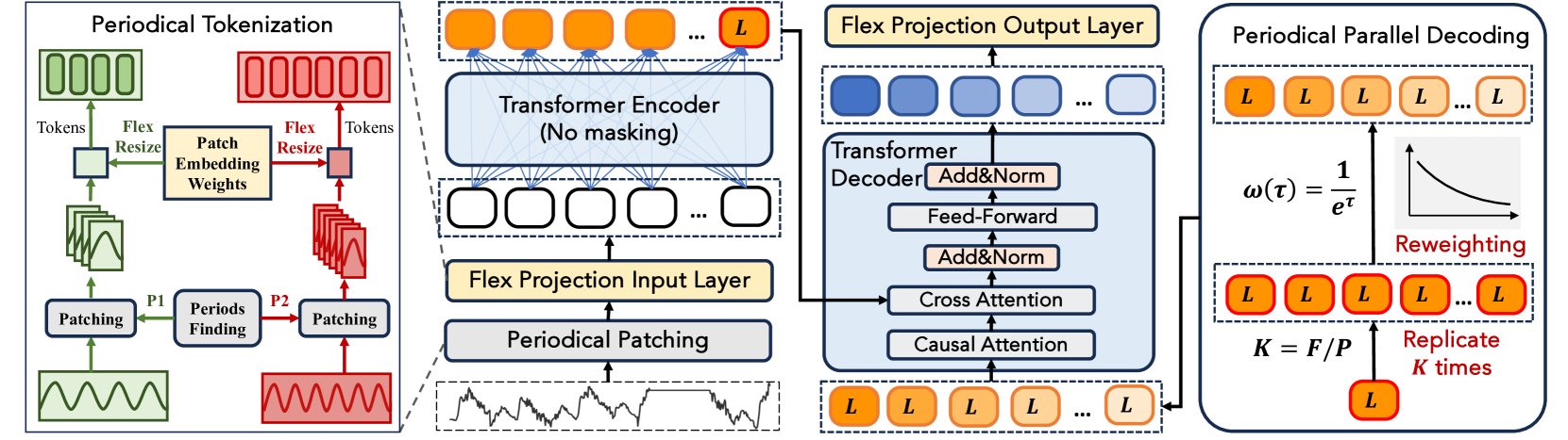
What makes the LightGTS model unique? It all starts with periodic tokenization — a true magical ruler that adapts to the rhythm of the series itself. The framework's authors suggest dividing the sequence into periodic patches — segments of data that correspond to a single complete cycle (such as a daily or weekly cycle). This operation is called Adaptive Periodical Patching. It takes into account the scale and structure of the time series and forms segments that fit perfectly into recurring patterns of market behavior.

To describe the method, we will consider a simple case — a one-dimensional time series. In practice, this easily scales to multivariate data: each channel is simply processed separately, without losing structure.

Let's imagine that we are working with a set of time series from various sources — financial assets, markets, and timeframes. Each series has its own internal rhythm — the so-called natural period. This could be, for example, a daily trading cycle, weekly volatility, or a seasonal trend. To work effectively with such series, the first step is to determine the length of this period — that is, how many time points in the data being analyzed make up one complete cycle.

If you have preliminary information about the data frequency (for example, if it arrives once an hour or once a minute), it is easy to determine the cycle length: for example, for a daily period with hourly data, this would be 24 data points. But if no frequency information is available, spectral analysis — including the Fast Fourier Transform (FFT) — comes to the rescue, helping to sniff out the dominant frequencies in the series. It is precisely these frequencies that reflect recurring patterns — cycles that are so important in forecasting market dynamics.

Once the cycle length — let's call it P — has been determined, the entire time series is neatly split into consecutive, non-overlapping fragments exactly one period long. Each such segment, or patch, contains P points and covers one complete cycle. The number of such patches is simply L divided by P, rounded down, where L is the length of the original series.

At first glance, this step seems simple, but in reality, it gives the model access to an entirely new level of semantic structure. Different timeframes, frequencies, and sources are now interpreted within a single, period-synchronized space. This eliminates noise caused by differences in data scale and allows the model to learn to identify patterns that actually recur from cycle to cycle — rather than simply adapting to local volatility.

It is precisely this method of splitting the series that makes it possible to train on heterogeneous data sources. Despite the difference in frequencies, they are all converted to a comparable form, where the period is the key unit of information. This means that the model can identify and generalize recurring market signals, which is critical for reliable forecasting in live trading conditions.

Once the time series has been split into cyclic patches, each covering a full cycle of the time series, it is important to map these patches correctly into a vector representation. This is where the magic of the projection layer begins, but, just like in real life, the devil is in the details.

A naive solution would be to use a fixed projection matrix that transforms each patch into a token. The problem? Different types of financial data have different cycle lengths: a daily cycle on minute candles consists of 1,440 points, while a weekly cycle on hourly candles consists of only 120. As a result, the input patches vary in size, and a fixed matrix simply cannot handle this: it either truncates the data or requires everything to be resized to a common size. Simple interpolation certainly helps — you can simply stretch or compress the data. But there is a catch: such operations distort the meaning. We end up with nicely aligned but empty tokens that do not mean much to the model.

To avoid such distortions, a flexible projection layer (Flex Projection Layer) is introduced. Its task is not simply to compress the patch to a fixed dimensionality, but to do so in a way that preserves the semantics of the data. In other words, the tokens derived from a patch of length 96 should be equivalent to those that would come from a patch of length 144, provided that both reflect the same market cycle.

How does this work technically? Suppose we have projection weights θ trained for a patch of length P. We want to adapt them for a new patch of length P′, in such a way that the product of the data and the weights (and thus the tokens) remains as close as possible. Simple interpolation will not work here — it is far too crude. Therefore, a linear transformation with weight adaptation via a pseudoinverse matrix is used — a method well known in numerical methods and regression analysis.

This mechanism is called flex-resize, and it solves an optimization problem: finding new weights θ′ that, when applied to new patches, produce a result as close as possible to the original — in terms of the Frobenius norm, to put it mathematically. A coefficient δ is introduced here — it accounts for the difference in variances between the original patch and the interpolated one, which helps maintain the statistical stability of the projections. The final formula for flex-resize looks quite complex, but it is essentially a clever way to make the weight matrix flexible and adaptive.

The Flex Projection Layer implementation uses two parameter matrices — one for input and one for output — each designed for a reference patch size (for example, 96). During the model’s forward pass, these matrices are adjusted to the required length of the current patch using that same δ⁻¹(A)+ transformation. After that, the patches are easily projected into the model’s hidden space — the tokens are ready and retain the full structure of the original market cycle.

Thus, regardless of whether the model analyzes a weekly trend using daily candles or scalps minute charts, it always works with data presented in a unified, consistent manner. This resolves the conflict between different scales and allows for the effective use of pre-trained weights without having to retrain from scratch. And in financial markets, where data come from various sources and at varying frequencies, such flexibility is not a luxury but a necessity.

The architecture of the LightGTS framework, like the classic Transformer, uses an Encoder and a Decoder, each of which includes multi-head attention modules and fully connected layers (Feed-Forward Networks). However, there is one key detail here — the attention modules use rotary positional encoding (RoPE), which allows them to take into account not only the absolute but also the relative positions of tokens. This is particularly relevant for time series where it is not just the order but the distance between points that matters.

After the periodic patches have been converted into tokens using Flex Projection, a sequence of tokens 𝐗ₑ = {𝐱ₑ₁, 𝐱ₑ₂, …, 𝐱ₑₙ} is formed, where each 𝐱ₑᵢ is a vector representation of the patch indexed by i. When processing this sequence, the Encoder adds positional structure using RoPE: tokens do not simply remember their own positions; they also take into account the relative offsets from one another.

Specifically, for each token, the query (Query) and key (Key) vectors are computed using the trainable matrices 𝐖Q and 𝐖K. Next, for the pair of vectors (𝐱ₑᵢ, 𝐱ₑⱼ), representing positions i and j, a rotation matrix 𝐑i−j is applied; it precisely encodes the difference between their positions. The resulting similarity measure between tokens i and j is calculated using the following formula:

The higher this value is, the more attention token i gives to token j. All such values are normalized using the SoftMax function and used to compute a weighted sum of Value vectors obtained via yet another trainable matrix 𝐖V.

It is precisely this attention that, quite literally, determines for each token which of its neighbors to look at and how intensely. After attention, each token is further processed by a fully connected block — a Feed-Forward Network — which extracts hidden features and enriches the representation.

As a result, the output of the Encoder is a latent space where each vector 𝐞ⱼ contains not only local information about the patch but also context from all other tokens, taking into account their relative positions in the time series. This mechanism allows the model to understand the structure, rhythm, and recurring patterns in the data, which is critical for financial time series, where it is not so much the individual data point that matters as its context.

As mentioned earlier, periodic patching helps extract recurring cycles from time series. However, to make the most of this information when generating a forecast, the model employs a new approach — periodic parallel decoding. Unlike the classical autoregressive approach, in which forecasts are constructed step by step, this method uses a non-autoregressive strategy that allows the entire future time horizon to be processed at once.

The key idea is simple yet elegant: the final token 𝐞ₙ from the Encoder’s output latent space contains compressed information about the entire preceding sequence, including its internal periodicity. Therefore, we take this particular token, clone it K times (where K = F/P — that is, the number of cycles to be forecast), and obtain the matrix 𝐇, which will serve as the input to the decoder.

However, it is important to note that the influence of the last token on forecasting weakens as we move further forward in time. Therefore, the weighting function ω(j) = 1/eʲ is applied to each cloned vector 𝐡ⱼ, exponentially reducing its contribution as the distance from the current moment increases. The resulting weighted tokens ω(j)·𝐡ⱼ are fed into the decoder simultaneously, which is the essence of the decoder’s parallel architecture.

The decoder outputs a matrix 𝐙 — forecast tokens corresponding to future cycles. To convert these tokens back into standard time-series values, the model uses inverse projection via the already familiar Flex-resize mechanism, this time applying it to the decoder parameters θd.

Thus, the model generates the entire forecast horizon 𝐘̂ all at once, without the error accumulation and delays typical of step-by-step prediction. This not only speeds up computations but also better preserves periodicity, since it was established as early as the tokenization stage and is now carried through the entire architecture — from the Encoder to the final output.

Under the hood, LightGTS runs like clockwork: rhythmically, precisely, and without unnecessary overhead. Thanks to periodic tokenization and parallel decoding, the model avoids the classic pitfalls of cumbersome architectures and poor transferability.

In accordance with established practice in time-series forecasting, the authors of the LightGTS framework use the classic Mean Squared Error (MSE) as the loss function. It measures the deviation between forecast values and actual observed data, serving as an objective criterion for forecast quality.

The authors' visualization of the LightGTS framework is shown below.

Implementation Using MQL5

After a detailed examination of the theoretical aspects of the LightGTS framework, we now move on to the practical part of our article. This section presents our own approach to implementing the key components of the model using MQL5 — taking into account the characteristics of financial time series and the platform's limitations.

Let's start with one of the most fundamental — and at the same time most interesting — elements: adaptive periodic patching. This mechanism is where the process of transforming a time series into a structure suitable for processing by a Transformer begins. We face several non-trivial challenges here.

One of them — dynamic changes in patch size — is already mentioned by the authors of the original framework. The paper proposes an elegant method for solving this problem using linear interpolation of weights. However, in practice, it addresses only part of the problem.

After all, if the patch size changes, the number of patches changes as well — dynamically and unpredictably. And this adds an extra layer of complexity to the model's architecture, especially when implementing it in a strictly typed language such as MQL5. Traditional loops and arrays require precise size control at all stages, which means it is necessary not only to adapt the dimensionality of the input data, but also to develop a mechanism for adaptively splitting the time series into a variable number of patches — while preserving their periodicity and consistency with historical observations.

Unfortunately, the architectural solutions we use do not allow dynamic dimensionality for input or output tensors at runtime. Therefore, we need a different, more pragmatic approach that provides fixed buffer sizes while still allowing us to work with a variable number of tokens.

One possible option is to create an overprovisioned buffer designed to accommodate the maximum possible number of tokens. If the actual number of tokens is smaller, the extra cells are set to zero. This approach does indeed provide a certain degree of flexibility when working with different numbers of patches; however, this flexibility comes at the cost of unnecessary memory consumption, a significant portion of which remains unused.

Furthermore, it is important not to overlook a key weakness of the Transformer architecture: the quadratic complexity of attention with respect to sequence length. The more tokens we feed in, the more time and resources will be required to process the attention blocks themselves. In other words, an excessive number of tokens is not only memory-inefficient but also directly harms the model’s computational performance, especially in real-time conditions or when processing arrays of high-frequency market data.

Therefore, there is a need for an alternative, more flexible approach. In this regard, the LightGTS framework’s concept of non-overlapping periodic patches, proposed by its authors, is worth noting; under this concept, each segment of the time series corresponds to a single complete cycle. This is quite logical: a time series often contains distinct periodic components, and analyzing each period separately allows us to extract semantically clean features.

However, we suggest looking at the problem from a different perspective. What if we were to abandon the strict requirement that patches not overlap? Instead, we can set the desired number of output patches and adjust the overlap length between adjacent windows depending on the periodicity of the input sequence.

This approach offers a number of advantages. First, it ensures a constant number of patches regardless of the periodicity of the time series being analyzed. This is extremely convenient when designing a fixed architecture. Second, flexible overlap allows for complete coverage of the cyclic data structure without truncating it or losing information between window boundaries. Finally, this makes it possible to control the resolution of the semantic representation more smoothly without compromising the compactness of the output tensor.

Simply put, we propose trading the strict “one patch — one cycle” rule for controlled representation density, while preserving the total amount of output information and increasing the model’s robustness to changes in the length of the input series.

I think the concept is clear. Now is the perfect time to move on to the practical implementation. The first step is to determine the periodicity of the time series being analyzed. To do this, we will use a classic, time-tested method based on the Fast Fourier Transform (FFT).

The essence of the approach is simple: we examine the amplitude spectrum of the frequency components of the time series and identify the frequency with the highest energy. This frequency typically corresponds to the dominant cycle in the data. The period, in turn, is calculated as the reciprocal of the detected frequency.

Why do we choose FFT specifically? First, it is a fast and efficient algorithm, even when working with large amounts of data. Second, it makes it possible to identify hidden periodic dependencies that may be impossible to detect visually. Finally, one of the advantages of FFT is that it enables us to work even when we lack a priori information about the frequency characteristics of a time series — which is often the case with real-world trading data.

And, of course, another bonus is the availability of a ready-made FFT implementation in our library. Let me remind you that we used it as part of our work with the FITS framework.

The FFT implementation in our library returns the real and imaginary parts of the spectrum, which fully matches the classical representation of the result of the fast Fourier transform. However, this information alone does not answer the question of which frequency dominates the signal and determines the structure of the oscillations.

To avoid overloading the CPU and maintain parallel efficiency, we implement a kernel that determines the dominant frequency for each individual sequence directly within the OpenCL context. Each work-item receives its own spectrum, calculates the energy of all frequency components, and selects the component with the maximum amplitude. It's like listening to a complex melody and instantly recognizing the underlying rhythm that gives it its structure. This approach is particularly important when working with multivariate time series, where each variable may have its own characteristic frequency.

We implement the algorithm within the OpenCL kernel MainFreq, which operates on arrays of real and imaginary spectral components. It returns an array containing the indices of the most prominent frequencies for each sequence.

__kernel void MainFreq(__global const float* freq_r,
                       __global const float* freq_im,
                       __global float *main_freq,
                       int dimension
                      )
  {
   if(dimension <= 0)
      return;
//---
   size_t n = get_global_id(0);
   const int shift = n * dimension;

In the kernel body, we first identify each work-item in a one-dimensional task space. The resulting index indicates the unique number of the individual sequence being analyzed. Using this index, we immediately determine the offset in the spectrum arrays so that each work-item processes only its own sequence.

Next, we initialize the variables to store the maximum amplitude (energy) and its corresponding index.

float max_f = 0;
float max_id = 0;
float energy;

This completes the preparatory work, and next we set up a loop over the spectrum, starting with the first harmonic.

for(int i = 1; i < dimension; i++)
  {
   float2 freq = (float2)(freq_r[shift + i], freq_im[shift + i]);
   energy = ComplexAbs(freq);
   if(max_f < energy)
     {
      max_f = energy;
      max_id = i + 1;
     }
  }

We intentionally skip the zero frequency (the DC component) — it does not carry information about periodicity, but instead reflects the constant component of the signal.

At each iteration, we construct a complex number from the real and imaginary parts. The modulus of this number represents the strength of the corresponding frequency. If the energy found exceeds the current maximum, we update the values.

Finally, after iterating through the entire spectrum, we write the result to the global data buffer.

 main_freq[n] = max_id;
}

The algorithm works like an experienced conductor, closely monitoring every instrument in the orchestra and determining which one is playing the lead part. We do not just find the frequency — we calculate the most prominent period of the signal, which is then used to adaptively construct patches in the model. And since each series (in a multimodal setting) is processed independently, we end up with a scalable, flexible, and fully autonomous system for determining local periodicity.

It is also worth emphasizing that the proposed algorithm is fully deterministic, contains no trainable parameters, and incurs no training costs. It relies exclusively on the physical nature of the spectrum: the amplitude of the frequency components is estimated directly, without using any statistics, regressions, or adaptive weights. This makes the method transparent, reliable, and particularly convenient during the data preprocessing stage — when it is critical to avoid introducing distortions associated with underfitting or overfitting. In other words, this approach relies on pure, unbiased mathematics rather than probabilistic assumptions, which is particularly important when analyzing volatile market time series.

The next step in our work will be the actual implementation of the adaptive patching algorithm with a dynamically changing segment size. However, as you can imagine, this is not something you can explain in a few words. Implementation requires attention to a multitude of technical details, and this article is already quite long as it is. Therefore, in the best tradition of suspenseful TV series, we suggest taking a short break and continuing our discussion of how to implement the proposed approaches in the next article.

In that article, we will walk through, step by step, how to implement a mechanism for dynamically generating patches that accounts for variable cycle lengths while maintaining a consistent number of output tokens. We will consider the possible trade-offs between architectural flexibility and computational efficiency.

Conclusion

In this article, we have examined the theoretical foundations of the LightGTS framework in detail, focusing on its key components: periodic patching, flexible token projection, and the parallel decoding mechanism. We analyzed how the architecture handles multivariate time series and adapts to different periods without having to retrain the model. Particular attention was paid to the technical aspects of calculating the dominant frequency using the fast Fourier transform.

We also discussed the practical limitations associated with dynamic memory allocation and a variable number of tokens, and proposed alternative solutions based on overlapping patches and a fixed-length output vector. This approach not only improves compatibility with the Transformer architecture, but also allows for more efficient use of resources, avoiding excessive memory consumption and performance degradation.

The material presented here serves as a solid foundation for the subsequent implementation of the full version of adaptive patching and its integration into the predictive architecture. In the next article, we will continue on this path, focusing on specific implementations of adaptive time-series segmentation and the integration of the resulting tokens into a trainable model.

References

• LightGTS: A Lightweight General Time Series Forecasting Model
• Other articles in this series

Programs used in the article

#	Name	Type	Description
1	Study.mq5	Expert Advisor	Expert Advisor for offline model training
2	StudyOnline.mq5	Expert Advisor	Expert Advisor for online model training
3	Test.mq5	Expert Advisor	Expert Advisor for testing the model
4	Trajectory.mqh	Class Library	Structure describing the system state and model architecture
5	NeuroNet.mqh	Class Library	Class library for building neural networks
6	NeuroNet.cl	Library	Code library for an OpenCL program