Neural Networks in Trading: Effective Feature Extraction for Accurate Classification (Building Objects)

Introduction

In the previous article, we explored the theoretical aspects of the Mantis framework — a foundation model for classifying time series that avoids the computational complexity of regression algorithms without sacrificing accuracy. It transforms the raw data from the sequence being analyzed into clear signals with well-defined confidence levels, offering a new level of analytical quality.

Imagine a classic forecasting model: it learns to minimize prediction error, but often fails in the face of sudden spikes in volatility. Such algorithms drift along with the market. They are difficult to adapt. They are susceptible to overfitting and do not provide transparent reliability estimates. We need more than just a prediction of a future value. We need real-time market-regime recognition, determining whether the price is moving according to a typical or anomalous scenario. This is where Mantis begins as a model trained not so much on regression as on understanding patterns.

Mantis is based on the idea of time series tokenization, borrowed from vision transformers. Instead of scanning tens of thousands of ticks or seconds, the time series is divided into a strictly defined number of patches. As a result, time series of different lengths are processed using the same number of steps, eliminating the need to reshape the architecture for different scales. Then comes the magic of hybrid attention: in one view, the model examines fine-grained local changes through convolutions and pooling, while in the second, it captures long-term trends using global attention. The combination of these two perspectives allows the model to simultaneously see the slightest fluctuations and sense the overall direction of movement.

The model's key secret ingredient is contrastive pretraining. Imagine two slightly distorted versions of a single segment of price history. Mantis learns to draw their embeddings closer in space, as if compressing several bands of light into a single beam, while simultaneously pushing completely different segments apart, like an electron and a positron. This contrast provides the model with a stable perception of the pattern, which is particularly valuable in the presence of changes in amplitude, small time shifts, or non-standard noise.

The process concludes with temperature scaling — the final calibration of the outputs. Traders are interested not merely in a “reversal/no reversal” verdict, but in the degree of confidence. Mantis can output not abstract scores, but plausible well-calibrated probabilities. Experience shows that if a model predicts an “80% probability of reversal,” then in reality, approximately 80 out of 100 such signals will turn out to be correct.

The true value of Mantis becomes apparent when multi-channel information is fed into it. The RSI dancing in rhythm, trading volumes, moving averages, and currency-pair correlations form a complex picture. Direct concatenation of these signals leads to an explosion in the number of parameters, while separate processing loses cross-dependencies. The solution in Mantis is lightweight adapters that compress inter-channel interactions, leaving only what matters most: the strength of the connection between indicators. The model saves memory, and the trader saves time on configuration.

To gain a deeper understanding of the Mantis architecture, let's walk through its steps. The first stage is the initial convolution: a time series with d channels passes through a layer with 256 output channels, forming a dense representation. The tensor is then divided into equal parts, and channel-wise mean pooling transforms the resulting data into 32 tokens, each carrying local information.

In parallel, a differential stream is constructed: first-order differences of the input data enhance sensitivity to short-term dynamics. The resulting data then follow the same patching process.

The third and fourth streams — the statistical streams — collect the mean and standard deviation of the input data within the same 32 windows, conveying the overall backdrop of volatility and level.

These four streams pass through separate linear projection layers to align their dimensionality, then are concatenated and projected into global tokens of the specified size.

A class token and sinusoidal positional encoding are added to the token sequence that encodes the sequence under analysis so that the model does not lose information about the order. The data are then fed into the transformer: 6 layers, multi-head attention with 8 heads, normalization, a two-layer FFN with GELU, and Dropout at 10% during training.

The model was trained in two stages. In the first, contrastive stage, it was trained on a combined corpus of ten public datasets: more than 7 million time series, 100 epochs, and a batch size of 2,048 on four NVIDIA Tesla V100 GPUs. This resembles an intensive training boot camp. In the second stage, a classification head is added and the outputs are temperature-calibrated. This two-phase approach makes it possible to achieve a combination that is rare for neural networks: high accuracy and reliable interpretability.

Finally, let's talk about flexibility. To handle tasks of different scales and tailor models to different budgets and data structures, the authors of the Mantis framework propose using several types of adapters:

• PCA and Truncated SVD are classic, time-tested methods of linear dimensionality reduction;
• Random Projection is a fast, simple, yet powerful way to reduce the dimensionality of a feature vector;
• Variance-Based Selector selects only the most informative channels based on variance;
• Differentiable Linear Combiner (LComb) is a trainable adapter that adapts to a specific task alongside the main model.

These adapters make it possible to balance speed and accuracy, conserve computational resources, and avoid losing critical inter-channel connections.

Ultimately, Mantis is not just a model, but an entire engineering suite for in-depth analysis of time series. Its strength lies not in grand statements, but in meticulous execution: careful attention to every patch, the careful integration of local and global contexts, rigorous calibration, and careful channel compression. This combination of analytics and artificial intelligence allows us to act with confidence, based on statistics and proven algorithmic principles, rather than relying on guesswork. In an era where speed and accuracy are everything, Mantis is the tool that helps you maintain your balance on the tightrope of the market.

An author’s visualization of the Mantis framework is shown below.

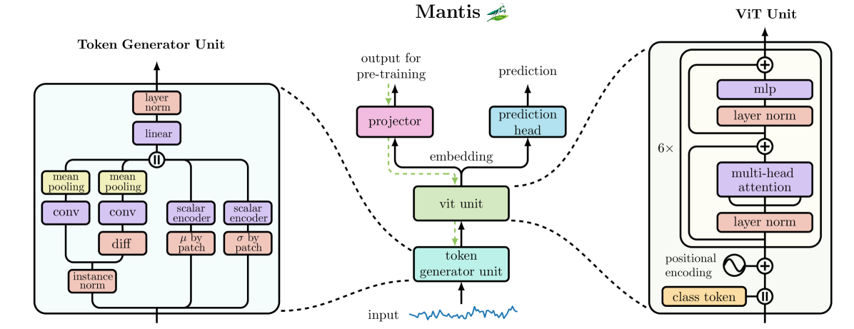
In the practical section of the previous article, we implemented a basic component for processing time series — the CNeuronConcatDiff module. This object combined the algorithm for calculating the first difference with a mechanism for concatenating tensors from different information streams. It marked the beginning of the practical implementation of the Mantis framework core.

Today, we will continue building this architecture by moving on to the next important building blocks of the neural network model. During the planning phase, in the previous article, we agreed on the need to implement temporal encoding in the data stream. This decision was driven by the desire to improve interpretability and account for the positional structure of the source data, without sacrificing performance. Of course, we are not going to reinvent the wheel: fortunately, we already have a time-tested object — CMamba4CastEmbedding. We developed it as part of our work on the Mamba4Cast framework, and now it is perfectly suited to this task.

The next logical step is to organize the patching of the time series. It is at this stage that the model loses its dependence on the length of the input sequence and gains the ability to operate on a fixed number of patches, regardless of the scale of the data. This is, without exaggeration, one of the most important modules in the classifier's architecture, since the stability of all subsequent processing depends on its implementation. That is where we will start today’s work: step by step, we will build a mechanism that splits the stream of source information into compact, informative patches.

Segmentation Object

The authors of the original Mantis framework approached the problem of time series segmentation from an unexpected but elegant angle. Instead of simply dividing the sequence into equal segments, they proposed first transforming the data using a convolution operation. What is more, they did not apply convolution merely for the sake of it, but used it to transform a one-dimensional time series into a multi-channel tensor. At first glance, this idea may seem unnecessary, but in practice it offers a significant advantage: by using a small-window convolution, the model begins to detect local signal fluctuations and capture important nuances in market behavior that might otherwise be lost against the backdrop of the overall trend.

After this transformation, we end up with a multi-channel tensor in which each channel represents a separate projection of the original time series — in other words, a “mini-representation” of the signal from its own perspective. This tensor is then evenly divided into a fixed number of patches. These are the patches — the building blocks that the model will work with going forward. And this is where the next stage comes into play: aggregating information within each segment.

The authors of Mantis proposed using the classic channel-wise averaging operation known as mean-pooling. It is simple, intuitive, and provides a good, smoothed representation of the segment. Unlike max-pooling, where only the maximum value is retained, mean-pooling preserves context, allowing each element of the time series to contribute to the final token. This is especially useful when each patch covers a fairly large portion of the data — in such cases, you need to take into account all the available information, not just the peaks and troughs. The tokens generated in this way provide a compact and informative representation of the temporal structure of the source data, suitable for further analysis by a transformer.

However, as practice shows, mean-pooling can be too “polite” — it averages not only the information but also any anomalies or sharp turns in the signal structure. For a foundation model, this may be an acceptable compromise: it remains simple, fast, and generalizable. But we decided to take it a step further. In our implementation, we replaced the standard mean-pooling with a combination of channel-wise convolution followed by max-pooling.

What does this give us in practice? First, the convolution operation extracts features within each channel, providing initial filtering and emphasizing local changes. Next, max-pooling highlights the most pronounced instances of these features. This approach makes the model more sharply tuned to the dynamics of the time series. Instead of averaging everything, it captures key features, which means it responds more quickly and accurately to sudden movements. This property becomes critically important in high-frequency trading or when working with volatile assets.

It is precisely thanks to this modification of the patching method that our classifier is able to adapt to the shape and structure of each specific time series. It no longer simply breaks data down into segments; it performs analysis, extraction, filtering, and evaluation. In such a system, a single patch is no longer just a fragment of a signal, but a full-fledged, information-rich token that carries both the context and the shape of the signal.

The proposed algorithm is implemented within the CNeuronMantisPatching class. This is a specialized module responsible for segmenting a time series into structured patches and generating a high-level representation suitable for further processing. This is where the real understanding of the data begins: local patterns are extracted from a simple one-dimensional stream and transformed into dense vector descriptions.

The CNeuronMantisPatching class is structured as a multi-stage computational pipeline. It contains several internal objects, each of which performs a highly specialized task. The class structure is shown below.

class CNeuronMantisPatching   :  public CNeuronTransposeOCL
  {
protected:
   CNeuronTransposeOCL     cToVarSeq;
   CNeuronConvOCL          cProjecting;
   CNeuronTransposeVRCOCL  cToVarProjSeq;
   CNeuronConvOCL          cPatchingProj;
   CNeuronProofOCL         cProof;
   //---
   virtual bool      feedForward(CNeuronBaseOCL *NeuronOCL) override;
   virtual bool      updateInputWeights(CNeuronBaseOCL *NeuronOCL)  override;
   virtual bool      calcInputGradients(CNeuronBaseOCL *NeuronOCL)  override;

public:
                     CNeuronMantisPatching(void) {};
                    ~CNeuronMantisPatching(void) {};
   //---
   virtual bool      Init(uint numOutputs, uint myIndex, COpenCLMy *open_cl,
                          uint count, uint patchs, uint variables,
                          uint embedding_size, uint patch_filters,
                          ENUM_OPTIMIZATION optimization_type, uint batch);
   //---
   virtual bool      Save(int const file_handle) override;
   virtual bool      Load(int const file_handle) override;
   //---
   virtual int       Type(void)  override const {  return defNeuronMantisPatching; }
   //---
   virtual void      SetOpenCL(COpenCLMy *obj) override;
   virtual bool      WeightsUpdate(CNeuronBaseOCL *source, float tau) override;
  };

All internal objects are declared statically, which allows the class constructor and destructor to be left empty. They are configured in the Init method, whose parameters provide a set of constants that allow us to unambiguously determine the architecture of the object being created.

bool CNeuronMantisPatching::Init(uint numOutputs, uint myIndex, COpenCLMy *open_cl,
                                 uint count, uint patchs, uint variables,
                                 uint embedding_size, uint patch_filters,
                                 ENUM_OPTIMIZATION optimization_type, uint batch)
  {
   if(!CNeuronTransposeOCL::Init(numOutputs, myIndex, open_cl, variables * embedding_size,
                                                        patchs, optimization_type, batch))
      return false;

It is worth noting that we expect the input to the CNeuronMantisPatching object to be a matrix of values from a multichannel time series, where each column represents a separate channel. Moreover, each channel consists of a sequence of numerical measurements over time. In other words, we are dealing with a matrix of dimension [T * C], where T is the number of time steps and C is the number of channels (variables).

Data transposition objects are used to enable independent processing of individual channels within the module. This is necessary to ensure separate processing along the channel and time axes — such isolation is difficult to achieve without explicitly moving the axes. Furthermore, the CNeuronMantisPatching class itself inherits from CNeuronTransposeOCL, which makes it possible to perform the inverse transposition using the parent class methods after all transformations have been applied, returning the output tensor in the expected form.

The first step of the initialization method is to call the method of the same name in the parent class, CNeuronTransposeOCL. This method prepares the basic structure and performs the preliminary initialization of the parameters. This step is necessary for all inherited mechanisms to function properly.

Once the parent class has been successfully initialized, configuration of the internal components begins. The first of these to be configured is the cToVarSeq object — a matrix transposition layer that provides convenient access to the individual time series of each channel. Its purpose is to transform the input data so that each channel becomes an independent time series suitable for further local convolution.

   int index = 0;
   if(!cToVarSeq.Init(0, index, OpenCL, count, variables, optimization, iBatch))
      return false;

Next, we initialize the local encoding object cProjecting. This is a convolutional layer that acts as an “attentive observer,” scanning each channel of the time series with a fixed window of width 3 and a stride of 1. Its task is to identify short-term local patterns and represent them in a space of fixed dimension embedding_size.

   index++;
   if(!cProjecting.Init(0, index, OpenCL, 3, 1, embedding_size, count - 2, variables,
                                                               optimization, iBatch))
      return false;
   cProjecting.SetActivationFunction(SoftPlus);

It is important to emphasize that processing remains strictly per-channel: each channel is analyzed independently, which allows the model to adapt to the individual characteristics of the signals. Furthermore, each channel has its own unique set of convolutional filters, which gives the process exceptional flexibility and accuracy.

The result of this operation is a tensor with dimensions [C * T' * D], where:

• C — the number of channels (features),
• T' — the resulting time-axis length after convolution with a window size of 3,
• D — the dimension of the new representation after encoding.

This tensor is a locally compressed and already partially structured form of the original data, which will serve as the basis for further segmentation and aggregation. This gives us a kind of condensed snapshot of the short-term dynamics within each feature — something that traditional methods of time series analysis are rarely able to capture without cumbersome and resource-intensive transformations.

Next comes the segmentation phase. And here, it's important to understand one subtle point. In our context, the segmentation operation itself involves dividing the data along the time axis — that is, breaking the sequence into segments of fixed length. However, in the previous step, the convolution result is represented as a tensor, where the time axis is the second dimension. For convenience in further processing and to align with the architecture of the subsequent layers, we need to rearrange the axes.

Therefore, we use a three-dimensional tensor transposition object, reordering the axes to place the dimensions in a form convenient for temporal segmentation. As a result, we obtain a tensor with the new structure [C * D * T'].

   index++;
   if(!cToVarProjSeq.Init(0, index, OpenCL, variables, count-2, embedding_size, optimization, iBatch))
      return false;

This data representation is convenient and logical: we can now work directly with the sequence over time, dividing it into equal segments, each of which will be treated as a separate semantic segment. This is in line with our original intention — to move from analyzing individual points to analyzing patterns.

It is in this new form that the tensor proceeds to the next stage, where the main operations of segmentation and information aggregation take place. The main task is to divide a time series into a fixed number of segments and extract an informative representation from each one. However, since initially we are given only the required number of segments (patchs), we first need to calculate the size of a single segment—how many time steps will fall into each patch.

Next, we initialize the cPatchingProj convolutional layer, which will perform the segmentation. It uses a window equal to the calculated patch size and slides along the time axis with the same stride, which ensures the creation of non-overlapping segments.

   index++;
   int patch_size = (int(count + patchs) - 3) / int(patchs);
   if(!cPatchingProj.Init(0, index, OpenCL, patch_size, patch_size, patch_filters,
                        patchs, variables * embedding_size, optimization, iBatch))
      return false;
   cPatchingProj.SetActivationFunction(SoftPlus);

It is important to note that, unlike simple mean pooling, this uses a full-fledged convolutional operation with multiple filters (patch_filters). This allows the model not merely to average information within a segment, but to extract the most relevant features from each segment by responding to characteristic local patterns.

After the tensor passes through the cPatchingProj layer, we obtain a four-dimensional tensor with shape [C × D × P × F], where:

• P — the number of segments (patches),
• F — the number of filters applied to each patch.

This tensor contains the enriched representations of each segment of each channel across all filters. However, further processing requires aggregating this data. This is where the max-pooling operation is applied along the last dimension — that is, along the filter axis F. This operation selects the most pronounced value along each dimension and makes it possible to discard redundant or weakly activated filters. After that, the tensor has dimensions [C × D × P].

   index++;
   if(!cProof.Init(0, index, OpenCL, patch_filters, patch_filters, 
            patchs*variables*embedding_size, optimization, iBatch))
      return false;
//---
   return true;
  }

The final data transformation is performed using the parent class, which we initialized earlier. Therefore, we conclude the method by returning the Boolean result of the operations to the calling program.

It is worth noting that the CNeuronMantisPatching architecture is designed to be highly modular. Each internal layer handles channels independently, making the architecture extremely scalable. Regardless of the number of channels being analyzed, the processing logic remains the same, since each channel is treated as an independent data stream.

Moreover, this independent structure allows computations to be effectively parallelized. Since all the neural layers used are implemented in OpenCL, they automatically utilize the available GPU or any other compatible computing device. This makes it possible to run hundreds of parallel threads simultaneously, each processing a separate channel without any noticeable time penalty.

We described the main logic of the CNeuronMantisPatching class and the interaction of its internal components in detail when analyzing the structure of the initialization method. It is in this method that all the key stages of processing a multichannel time series are built up sequentially: from the initial transposition to segmentation and information aggregation.

To avoid overloading this article with unnecessary details, we have deliberately omitted descriptions of the forward (feedForward) and backward (calcInputGradients, updateInputWeights) passes. They implement strictly sequential calls to the identically named methods of the internal objects, corresponding to the architecture of the constructed pipeline.

The complete source code for this class, including the implementation of all helper methods, is provided in the attachment. If they wish, readers can review it on their own and explore all the technical details in greater depth.

Attention Module

In accordance with the general logic of the Mantis framework, the preprocessed time series sequence — already in the form of tokens composed of patches from individual channels — is fed into the Transformer module. This is where the final processing of temporal and cross-channel information takes place: a special class token is added to the token sequence, and positional encoding is incorporated.

The class token serves as a kind of information aggregator. While passing through the six layers of the multi-head self-attention (Self-Attention) mechanism, it aggregates structural information about the entire sequence. The corresponding output vector is interpreted as the class identifier of the analyzed time series — whether the task is recognizing a market phase, classifying indicator states, or forecasting the type of future movement.

In our implementation, we made certain adjustments to this stage. First of all, positional encoding was excluded. The reason is that the temporal structure of the sequence is already explicitly encoded in the tokens themselves, thanks to the built-in temporal encoding borrowed from the Mamba4Cast architecture. This approach allows the absolute and relative positions of each element within the channel to be encoded without resorting to sinusoidal or learned positional vectors, as is common in classical Transformers.

This change offers two advantages at once. First, it makes the model less sensitive to shifts and distortions in the input sequence. Second, it eliminates the conflict between the fixed positional code and the actual temporal context already present in the data. When applied to real market time series, this improves the model's robustness and allows the Transformer to focus on the content of the input signal.

In addition, in the author's implementation of Mantis, at the output of the Transformer only the class token is used — a special vector designed to accumulate generalized information about the sequence. This token is prepended to the input sequence, passes through all layers of the transformer, and is extracted at the output.

However, in our implementation, we opted for an alternative solution. Instead of the traditional method of inserting a class token at the beginning of the sequence and then extracting it, we use a cross-attention module (Cross-Attention). What makes it unique is that the class token is provided as the main query (query), while the tokens from the source sequence are provided as context (keys and values). This configuration allows the class token to focus on the most significant elements of the sequence, minimizing noise and strengthening relevant connections.

Furthermore, we applied a cross-attention variant with independent channels, in which each channel is analyzed in isolation. This makes it possible to assess the contribution of each channel to attention individually. This approach is particularly useful when analyzing multimodal or heterogeneous signals, as it prevents one channel from dominating the others and provides an objective, aggregated view of the entire structure of the time series.

Thus, the final container vector produced by the cross-attention block already contains a generalized and balanced representation of the entire temporal structure, suitable for subsequent classification or prediction.

From a technical standpoint, all of this is implemented in the CNeuronMantisAttentionUnit class, which inherits from CNeuronSoftMaxOCL. This means that the output immediately gives us the probability that the sequence being analyzed belongs to a particular class. The structure of the new object is shown below.

class CNeuronMantisAttentionUnit :  public CNeuronSoftMaxOCL
  {
protected:
   CNeuronBaseOCL                cClassToken[2];
   CNeuronMVCrossAttentionMLKV   cAttention;
   //---
   virtual bool      feedForward(CNeuronBaseOCL *NeuronOCL) override;
   virtual bool      updateInputWeights(CNeuronBaseOCL *NeuronOCL)  override;
   virtual bool      calcInputGradients(CNeuronBaseOCL *NeuronOCL)  override;

public:
                     CNeuronMantisAttentionUnit(void) {};
                    ~CNeuronMantisAttentionUnit(void) {};
   //---
   virtual bool      Init(uint numOutputs, uint myIndex, COpenCLMy *open_cl,
                          uint token_size, uint window, uint window_key, uint heads,
                          uint units_count, uint layers, uint variables,
                          ENUM_OPTIMIZATION optimization_type, uint batch);
   //---
   virtual bool      Save(int const file_handle) override;
   virtual bool      Load(int const file_handle) override;
   //---
   virtual int       Type(void)  override const {  return defNeuronMantisAttentionUnit; }
   //---
   virtual void      SetOpenCL(COpenCLMy *obj) override;
   virtual bool      WeightsUpdate(CNeuronBaseOCL *source, float tau) override;
  };

Inside the new class, we see two main components:

• cClassToken[2] — a two-layer MLP for generating a trainable class token;
• cAttention is the multilayer cross-attention object itself.

All internal objects are declared statically, which allows the class constructor and destructor to be left empty. As usual, internal objects are initialized in the Init method.

bool CNeuronMantisAttentionUnit::Init(uint numOutputs, uint myIndex, COpenCLMy *open_cl,
                                      uint token_size, uint window, uint window_key,
                                      uint heads, uint units_count, uint layers, uint variables,
                                      ENUM_OPTIMIZATION optimization_type, uint batch)
  {
   if(!CNeuronSoftMaxOCL::Init(numOutputs, myIndex, open_cl, token_size, optimization_type, batch))
      return false;

Here, we first call the method of the same name in the parent class, where, as you know, the initialization of inherited objects and interfaces has already been handled. After the parent class method has completed successfully, we move on to initializing the internal objects. First, we initialize the MLP for generating a trainable class token. The first layer always has a single element with a fixed value, while the second layer uses trainable parameters to generate a class token of the required size.

   int index = 0;
   if(!cClassToken[0].Init(token_size, index, OpenCL, 1, optimization, iBatch))
      return false;
   if(!cClassToken[0].getOutput().Fill(1))
      return false;
   index++;
   if(!cClassToken[1].Init(0, index, OpenCL, token_size, optimization, iBatch))
      return false;
   cClassToken[1].SetActivationFunction(SIGMOID);

To obtain token elements within a specified range of values, we use a sigmoid activation function on the final layer.

The next step is to initialize the cross-attention block. We receive all configuration data from the user in the parameters of our initialization method.

   index++;
   if(!cAttention.Init(0, index, OpenCL, token_size, window_key, heads * variables, window,
                       heads, 1, units_count, layers, 1, 1, variables, optimization, iBatch))
      return false;
//---
   return true;
  }

And we complete the method by returning the Boolean result of the operations to the calling program.

The feedForward method is equally concise. In the method parameters, we receive a pointer to the context object of the sequence being analyzed and immediately check its validity.

bool CNeuronMantisAttentionUnit::feedForward(CNeuronBaseOCL *NeuronOCL)
  {
   if(!NeuronOCL)
      return false;

Next, we need to generate the class token. However, this operation is performed only during model training. During operation, the model's parameters do not change; consequently, the class token remains fixed. And we do not need to regenerate it at every iteration.

//---
   if(bTrain)
     {
      if(!cClassToken[1].FeedForward(cClassToken[0].AsObject()))
         return false;
     }

The generated class token, along with the context of the sequence being analyzed, is fed into the attention block.

   if(!cAttention.FeedForward(cClassToken[1].AsObject(), NeuronOCL.getOutput()))
      return false;

The output of the attention block — an enriched class token — is passed to the input of CNeuronSoftMaxOCL, the parent class. This step converts the predicted value into a probabilistic interpretation. The result is a probability distribution over classes.

   if(!CNeuronSoftMaxOCL::feedForward(cAttention.AsObject()))
      return false;
//---
   return true;
  }

In conclusion, we note that the backward-pass methods (calcInputGradients and updateInputWeights) implement sequential calls to the corresponding functions of the nested components. Readers can explore their implementation on their own to fully understand the process of training and updating weights in the CNeuronMantisAttentionUnit module. The complete code for this class and all of its methods is provided in the attachment.

We completed all the work scheduled for today. In the next article, we will examine the architecture of the models and evaluate the effectiveness of the implemented solutions using real historical data.

Conclusion

We have gone all the way from initial data preparation — calculating first differences, concatenating features, and temporal encoding based on CMamba4CastEmbedding — to complex patch processing and intelligent aggregation via cross-attention using the class token. Each step in this chain — from transposition and local convolutions to max-pooling and multi-head attention — has been carefully designed to preserve as complete a picture of temporal dynamics as possible while optimizing computational resources with an emphasis on OpenCL parallelism.

As a result, we ended up with a modular architecture in which it is easy to adjust the number of channels, patch size, embedding depth, and number of attention heads without changing the underlying logic. This makes it possible to quickly adapt the model to a wide variety of financial scenarios — from high-frequency trading to the analysis of long-term trends.

In the next part, we will present a complete diagram of the trainable model based on the components described and show its results on historical data.

References

• Mantis: Lightweight Calibrated Foundation Model for User-Friendly Time Series Classification
• Other articles in this series

Programs used in the article

#	Name	Type	Description
1	Research.mq5	Expert Advisor (EA)	Expert Advisor for collecting examples
2	ResearchRealORL.mq5	Expert Advisor (EA)	Expert Advisor for collecting examples using the Real-ORL method
3	StudyContrast.mq5	Expert Advisor (EA)	Expert Advisor for contrastive encoder training
4	Study.mq5	Expert Advisor (EA)	Expert Advisor for offline model training
5	StudyOnline.mq5	Expert Advisor (EA)	Expert Advisor for online model training
6	Test.mq5	Expert Advisor (EA)	Expert Advisor for model testing
7	Trajectory.mqh	Class Library	Structure for describing the system state and model architecture
8	NeuroNet.mqh	Class Library	Class library for building neural networks
9	NeuroNet.cl	Library	OpenCL Program Code Library