Trends and Traditions: Using Rademacher Functions in Trading

Introduction

Modern trading requires high speed, accuracy, and adaptability. As a result, the need for advanced data analysis methods has increased significantly. However, traditional approaches often prove insufficiently effective for extracting useful information from noisy and nonlinear financial time series. In this article, we will explore the capabilities of Rademacher functions — powerful mathematical tools that have proven effective in signal processing and data analysis, but are not yet widely used in trading.

In this article, we will try to apply these functions to solve the following tasks:

• noise filtering and identification of significant trends;
• identifying patterns in price changes;
• time series forecasting;
• adapting to changing market conditions and developing trading strategies capable of responding flexibly to market changes.

The main purpose of this article is to demonstrate how the use of Rademacher functions can help traders and trading system developers address these issues.

Expected results include:

• an evaluation of the effectiveness of Rademacher functions for analyzing and processing market data;
• specific examples of how these functions are applied in trading, including algorithms for filtering, forecasting, and adapting to market conditions;
• testing these algorithms on historical data and examples of trading strategies built on these functions.

I hope you have already read the introductory article on Rademacher and Walsh functions. This article will serve as a starting point for the broader implementation of these functions in trading practice and will help create more sophisticated and adaptive trading systems.

Limitations and Capabilities of Rademacher Functions

If we ask ourselves how many methods for processing and analyzing time series exist today, the answer that comes closest to the truth would be: a great many. However, before putting them into practice, it is advisable to familiarize yourself with their limitations and drawbacks. As an example, let's take systems of Rademacher functions. Their first drawback is that they are incomplete. This means that it is impossible to accurately reconstruct the original signal using them. Another drawback of these functions is their strictly defined periodicity. The period of the functions can only be equal to some power of 2. All of these shortcomings may limit the practical application of these functions.

But as we know, our strengths are an extension of our weaknesses. And we can easily prove this claim using Rademacher functions. These functions are incomplete solely because they are constructed using the odd sine function. However, a linear trend can also be expressed using an odd function.

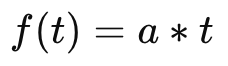
This means that Rademacher functions can be used to describe linear trends with considerable accuracy, which is their undeniable advantage. Traders love trends.

Now, let's discuss the period of Rademacher functions. Let's say I have decided to build a system of order 2. In the classical approach, the period of all functions will be 4. Let's say I decided to double the period (not the best example, but let's go with it). There is nothing preventing this. And what will this doubling achieve? It will have the greatest impact on the highest-order function. In the classical system, this function alternates between +1 and -1. It will only work well when there is a clear trend. After doubling, the coefficients of this function will look like this: +1, +1, -1, -1, and so on. This way, I can smooth this function, making it less sensitive to noise and outliers.

Note: If you are invited to an international conference on digital signal processing tomorrow, do not talk about this approach there — your proposal will be met with mixed reactions. And if you visit a local traders' club, the members will like this idea.

Now let's take a look at how this approach can be put into practice. First, we need to specify the order of the function system, P. Next, we will set the scale parameter M. In that case, the period of the functions can be calculated using the formula:

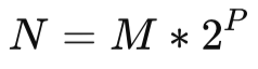
Of course, the indicator period cannot be arbitrary, but we do have some leeway in choosing it. The calculation of function coefficients remains the same.

Let's see how an indicator built using this method will behave. For this example, I set the parameters P and M to 3. The indicator divides the entire price range into 8 levels, each with a length of 3 bars.

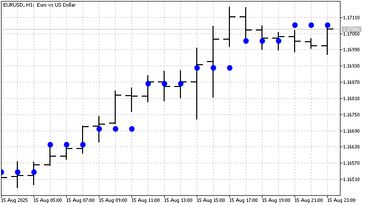
Each of these levels provides its own local price smoothing. However, what interests us most is the fact that all prices are involved simultaneously in the formation of each level. Therefore, we can regard them as a kind of support and resistance levels. Let L be the number of prices below a given level. Then its resistance strength can be calculated as follows:

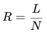
The greater the resistance, the weaker the support at that level, and vice versa. In a more familiar form, this indicator would look like this:

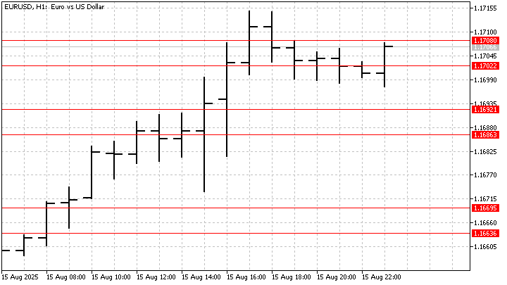
The main difference between these levels is that they are based on trend functions. This means that they are influenced not only by the prices themselves, but also by the order in which they follow one another. If you swap just two prices, the level values can change quite significantly. This indicator can be used as a filter. Now let's try some more complex ways of using Rademacher functions.

Forecasting Using Rademacher Functions

Up until now, we have been dealing with a system of functions. At the same time, we did not pay attention to the behavior of each function individually. Let's see what values a particular function can take in historical data. As an example, I will consider a first-order Rademacher function. When collecting statistics, I will not normalize the function values; I will convert the results into points. That way, I will get integers, and working with them is very simple and convenient. I am interested in what values the function can take and how often those values occur in the historical data. As a result, I will obtain an empirical probability density function (PDF), which in this case looks like this:

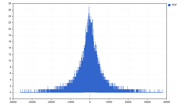
Based on the statistics we have collected, we can already draw some conclusions. As you can see, some values occur more frequently, while others occur less frequently. The first conclusion we can draw is that large trends occur less frequently than small ones. In addition, based on the PDF, we can construct a cumulative distribution function (CDF). From a mathematical standpoint, the CDF is the sum of the probabilities of the current value and all values below the current value. As a rule, it takes the form of an S-shaped curve that rises from 0 to 1.

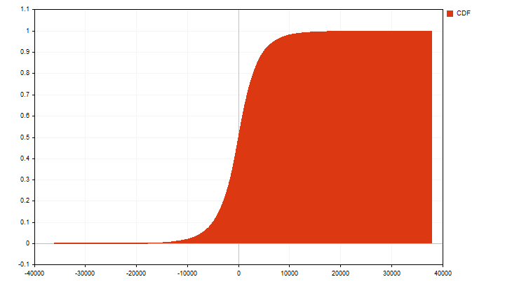
The main feature of the CDF is that it shows the probability that a value will be less than or equal to a given value. This feature can already be used in trading. For example, if the current CDF value is close to 0 or 1, this may signal the end of a trend and a possible change in its direction. And crossing the 0.5 level can serve as trend confirmation.

Let's take a look at how these functions can be used in practice. Let's assume that you are using an SMA with a period of N. You know the current value of this indicator. And what will it be after N bars? The answer to this question isn't as complicated as it seems at first glance. First, we need to find out how SMA values change over time. To do this, we need to collect statistics of this form:

Now let's recall that SMA coefficients are determined as follows:

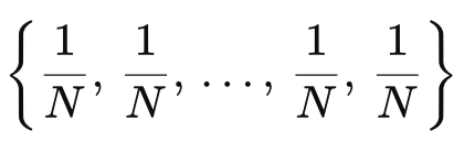
If we remove the normalizing factor, the difference between two SMAs will become a first-order Rademacher function with a period of 2*N. And we already know how to collect statistics for functions like these. So, our procedure will be as follows:

• Set the SMA period and the desired forecast accuracy;
• Calculate the coefficients of the first-order Rademacher function with a doubled period:
• Collect statistics for this function and construct the CDF;
• Using the CDF, find the minimum and maximum values that will correspond to the required forecast accuracy;
• Find the current SMA value. Using this value, along with the minimum and maximum from the previous step, we make a forecast.

An indicator built using this algorithm looks like this:

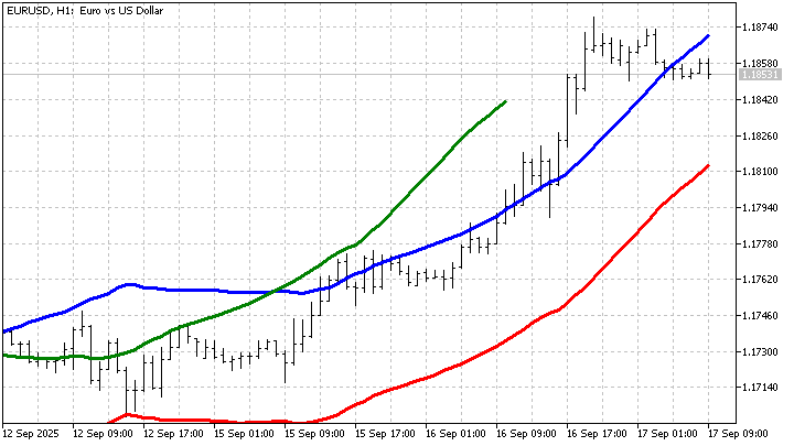
There is a 50% probability that the future value of the SMA will fall between the red and blue lines. The green line shows the future value of the SMA at the time the forecast is calculated. Of course, the indicator does make mistakes, but after all, the future is not predetermined.

Making the Model More Complex

Estimating future SMA levels is useful. But the ability to forecast the future trend value looks much more appealing. You will agree that if I tell you the price will rise over the next N bars, such a forecast would be preferable to some specific levels. But to be able to make such a forecast, we will have to put in a little effort.

First, we need to build an oscillator based on Rademacher functions. It will differ slightly from classic oscillators. Let's take a look at what the difference is. For example, suppose we decided to build an oscillator based on the SMA. All we need to do in this case is calculate the difference between the current price and the SMA value.

The Rademacher functions, however, are windowed. A change in the latest price causes all the function values to change across their entire period. On the one hand, this could be a drawback — traders might say that the indicator repaints. On the other hand, this is an advantage of these functions: they respond flexibly to the current market situation.

To build an oscillator, I will take advantage of these functions' ability to smooth out trends. The algorithm for calculating the oscillator will be as follows. First, I will find the values of all the Rademacher functions. After that, I will calculate the differences between the current price and the values of these functions. The sum of these differences will be the current value of the oscillator. As a result, I will end up with a model of trend change.

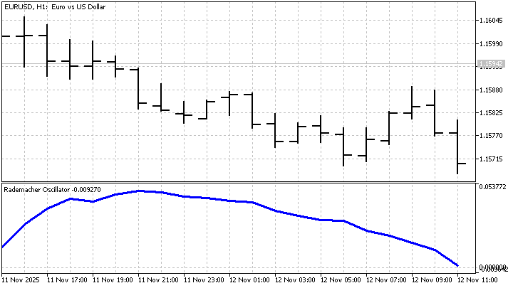
Now I am faced with the question: how can I obtain a forecast of the trend value from this model? To build a forecast, I will use Markov chains. These chains were first studied by A. Markov in 1906 in the article “On the Limit Distribution of a Class of Correlated Random Variables.” The essence of these chains is that they can be used to forecast the probability of a process transitioning from one state to another.

Let's assume I distinguish between three market states: uptrend, flat, and downtrend. Based on historical data, I can track how these states have changed and calculate the probability of the market transitioning from one state to another. These probabilities are most conveniently represented as a matrix.

	uptrend	flat	downtrend
uptrend	0.4	0.3	0.3
flat	0.3	0.4	0.3
downtrend	0.2	0.4	0.4

The left column of this matrix shows the possible current market states. The top row shows the market states at the next step. The table cells show the transition probabilities from one state to another.

This is the transition matrix of a Markov chain. Using this matrix, I can forecast the future market state. The matrix itself provides a forecast one step ahead. What should I do if I want to get a forecast two steps ahead? To do this, I need to multiply the transition matrix by itself.

Next, I want to see what happens at the third step. No problem. All I need to do is multiply the resulting matrix by the transition matrix.

As you may have guessed, by continuing this sequence of multiplications, I can make a forecast for any number of steps ahead. It is precisely this property that I will use to develop a trading strategy.

To describe the market state, I will use the Rademacher oscillator. Based on historical data, I will determine the maximum and minimum values of this indicator. I will distinguish between N states of the oscillator. In that case, the size of each state can be found using the formula:

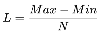
Now I can calculate the index of the state the indicator is in:

Next, I need to create an N×N matrix in which I will record the indicator's transitions from one state to another. For example, the indicator is currently in state I, and its next state will be J. Then I will increment the matrix element with those indices by 1. Using this matrix, I will create a transition probability matrix. To do this, I will find the sum of all the elements in a single row, and then divide each element in that row by that sum.

Knowing the probability values, I can forecast changes in the indicator state for any number of steps ahead. I will base my strategy on this forecast. The rules will be as follows:

• if the forecast indicates that the indicator state will increase, I will open a buy position;
• if the indicator state is expected to decrease, I will open a sell position;
• Positions are closed based on opposite signals.

Despite the simplicity of this strategy, its results look promising.

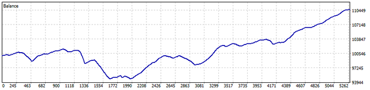
The main challenge with this strategy is that the trader must select not only the indicator parameters but also the parameters of the Markov chain. The results depend on the number of states. If there are only a few states, the chain will be too generalized and will have difficulty distinguishing market conditions. In this case, increasing the number of states could have a positive effect on the results. On the other hand, increasing the number of states may reduce the predictive ability of the chain.

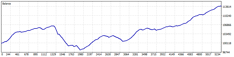
The use of Markov chains allows for more flexible approaches to position management. I used forced position closure, but another option is certainly possible. Let's assume that the forecast indicates that a price increase is unlikely or will be modest. In that case, instead of closing the buy positions, you can start managing them with a trailing stop. At the next step, the likelihood of a price increase has risen — you can disable the trailing stop.

Conclusion

This article has shown that Rademacher functions can be used to analyze and forecast financial time series. Methods for filtering out noise, identifying trends, and developing trading strategies based on these functions were examined.

A new approach to scaling the period of Rademacher functions opens up new possibilities for adapting to various market conditions. An indicator for support and resistance levels based on trend functions can take into account not only prices but also the order in which they occur, which can be useful when making trading decisions.

CDF-based forecasting and SMA adaptation using Rademacher functions have shown promising results, despite the simplicity of their implementation. The use of Markov chains to forecast the market state based on the Rademacher oscillator also yielded encouraging results when testing the trading strategy.

Despite some limitations of Rademacher functions, their sensitivity to trends and their ability to adapt flexibly to market conditions make them a valuable tool for market analysis.

The following software were used in preparing this article.

Name	Type	Description
Rademacher Trend	indicator	The indicator smooths the trend using Rademacher functions with an increased period. P - maximum order of the functions (valid values: 1–10) M - multiplier for increasing the period of the functions (minimum value: 1).
Rademacher RS	indicator	The indicator displays the levels of the Rademacher functions
Trend PDF	script	The script computes the PDF and CDF for Rademacher functions. The images are saved in the "Files" folder.
SMA Forecast	indicator	The indicator forecasts the future value of the SMA. PeriodSMA - SMA period Percent - forecast accuracy
Rademacher Oscillator	indicator	The indicator calculates the deviation of the current price from the smoothed trend
EA Rademacher Markov	Expert Advisor	The Expert Advisor implements a trading strategy based on the Rademacher oscillator and Markov chains. P - maximum order of functions M - period increase multiplier N - number of chain states (at least 3) Forward - number of forecasting steps (at least 1) OpenLvl - minimum number of states between the forecast and the current state for opening positions