

Neural Networks in Trading: Decomposition Instead of Scaling (Conclusion)
 174
174
 0
0

Introduction
Today's financial markets are not just a place where buyers and sellers meet, but a complex, dynamic ecosystem where every price tick is the result of the instantaneous interaction of hundreds of factors. There is no room here for chance in the usual sense of the word: behind the apparent chaos lie patterns, albeit ones clothed in complex, multilayered forms. It is precisely the ability to recognize these hidden patterns and anticipate their development that determines the success of a trader or an algorithmic system. In previous articles, we became acquainted with the SSCNN (Spatial-Sequential Convolutional Neural Network) framework. Behind this title — which may seem cumbersome at first glance — lies a very coherent and elegant concept that integrates spatial and temporal dependencies into a single computational algorithm.
The SSCNN is based on the idea that a time series is a time-unfolded representation of multidimensional processes. Every moment in time is connected not only to the past and the future, but also to parallel structures — internal feature spaces that change either synchronously or with a delay.
To capture these relationships, the model uses a cascade of blocks capable of extracting local patterns and sequential processing modules that retain and accumulate context. The key component here is the Attention-based Normalization module — a combination of attention and normalization that allows the system to focus on truly significant data segments while stabilizing the learning process. Thanks to this architecture, the SSCNN is capable not only of analyzing signals at different levels of detail, but also of adapting to changing data structures — which is particularly important for financial instruments, given their unstable volatility and changing market regimes.
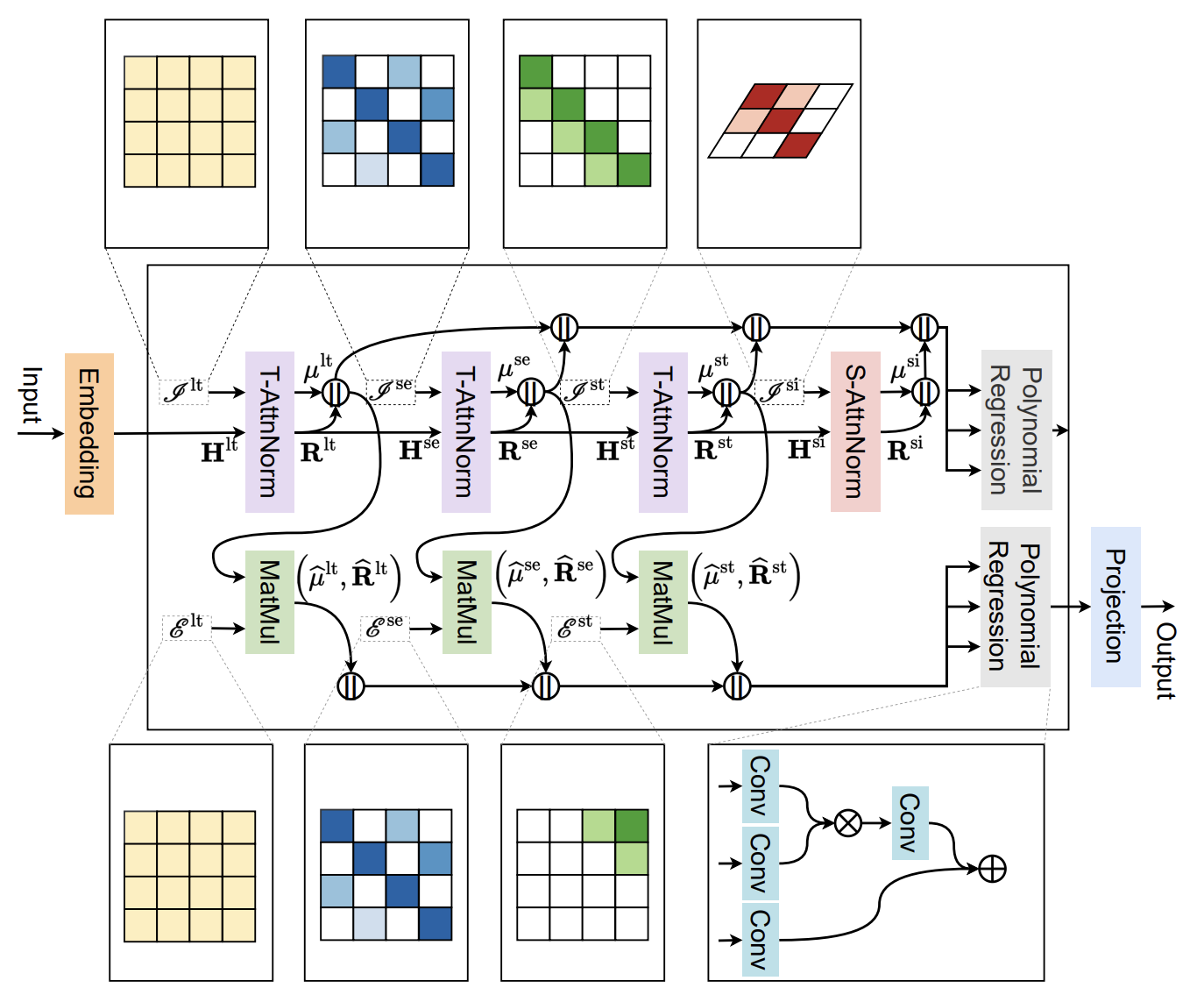
Another important advantage is its modularity. The SSCNN architecture is easily scalable and can be tailored to a specific task — whether it is short-term price momentum forecasting or identifying long-term cycles. The concept of layered data perception, in which each level of the model extracts its own set of features and passes them on to the next level, provides flexibility and robustness.
In previous articles, we examined in detail how these ideas were implemented in code and integrated into the MQL5 environment, laying the groundwork for a full-fledged trading system.
Now we are approaching the final stage, where theory must meet practice in its most demanding form. We will assemble the individual components into a cohesive framework architecture and evaluate how SSCNN processes and interprets market data. We will test the effectiveness of the implemented solutions under conditions that closely approximate real trading. This step is important not only for measuring forecast accuracy or the model’s stability, but also for understanding how deeply its algorithms sense the market, distinguish hidden structures, and recognize shifts in context. After all, the success of any trading system is ultimately determined not by the sophistication of its architecture, but by how well it handles noise, unexpected spikes, and treacherous turns in the charts.
Encoder
In previous articles, we built the individual blocks of the SSCNN architecture, and today we begin to combine them into a single Encoder — the very node where a multitude of information streams (long-term trends, seasonal patterns, short-term fluctuations, and spatial relationships) are carefully decomposed, organized, projected onto a specified forecast horizon, and then merged into a unified forecast representation.
The CNeuronSSCNNEncoder class implements this idea in code. Its task is not simply to call a set of modules sequentially, but to synchronize their operation: to isolate each component according to its own logic, extrapolate it to the required horizon, forecast the corresponding statistics, and only then assemble all of this into a rich, structured representation for the final polynomial regression. The Encoder manages data streams, organizes transpositions where necessary for correct phase-based operation, and ensures that each result from a separate subsystem ends up in its proper concatenation position in the required format. The class structure is shown below.
class CNeuronSSCNNEncoder   :  public CNeuronTransposeOCL
  {
protected:
   CNeuronPeriodNorm       cLongNorm;
   CNeuronConvOCL          cLongExtrapolate;
   CNeuronTransposeOCL     cLongMeanSTDevTransp;
   CNeuronBaseOCL          cLongMeanExtrapolate;
   CNeuronTransposeVRCOCL  cSeasonTransp;
   CNeuronAttentNorm       cSeasonNorm;
   CNeuronTransposeVRCOCL  cUnSeasonTransp;
   CNeuronConvOCL          cSeasonExtrapolate;
   CNeuronConvOCL          cSeasonMeanExtrapolate;
   CNeuronAttentNorm       cShortNorm;
   CNeuronConvOCL          cShortExtrapolate;
   CNeuronConvOCL          cShortMeanExtrapolate;
   CNeuronSAttentNorm      cSpatialNorm;
   CNeuronConvOCL          cSpatialExtrapolate;
   CNeuronConvOCL          cSpatialMeanExtrapolate;
   CNeuronBaseOCL          cConcatenated;
   CNeuronTransposeOCL     cTranspose;
   CNeuronPolynomialRegression   cFusion;
   //---
   virtual bool      feedForward(CNeuronBaseOCL *NeuronOCL) override;
   virtual bool      updateInputWeights(CNeuronBaseOCL *NeuronOCL)  override;
   virtual bool      calcInputGradients(CNeuronBaseOCL *NeuronOCL)  override;

public:
                     CNeuronSSCNNEncoder(void) {};
                    ~CNeuronSSCNNEncoder(void) {};
   //---
   virtual bool      Init(uint numOutputs, uint myIndex, COpenCLMy *open_cl,
                          uint units_count, uint variables, uint forecast,
                          uint season_period, uint short_period,
                          ENUM_OPTIMIZATION optimization_type, uint batch);
   //---
   virtual bool      Save(const int file_handle) override;
   virtual bool      Load(const int file_handle) override;
   //---
   virtual int       Type(void) override const  {  return defNeuronSSCNNEncoder; }
   virtual void      TrainMode(bool flag) override;
   virtual void      SetOpenCL(COpenCLMy *obj) override;
   //---
   virtual bool      WeightsUpdate(CNeuronBaseOCL *source, float tau) override;
   virtual void      SetActivationFunction(ENUM_ACTIVATION value) override { }
  };
The processing chain inside the Encoder is carefully arranged. All internal objects are declared statically, so the class constructor and destructor remain empty, and the actual construction of the computational graph is performed centrally in the Init method.
bool CNeuronSSCNNEncoder::Init(uint numOutputs, uint myIndex, COpenCLMy *open_cl,
                               uint units_count, uint variables, uint forecast,
                               uint season_period, uint short_period,
                               ENUM_OPTIMIZATION optimization_type, uint batch)
  {
   if(!CNeuronTransposeOCL::Init(numOutputs, myIndex, open_cl, units_count + forecast,
                                variables, optimization_type, batch))
      return false;
   activation = None;
The method’s algorithm begins by initializing the parent class CNeuronTransposeOCL, to which the basic parameters of the architecture being created are passed. This call sets up the general infrastructure: allocating global buffers, setting tensor sizes, and binding the OpenCL context.
Note that the dimensionality of the results tensor is specified as the sum of the length of the analyzed sequence and the forecast horizon. Here it becomes clear that, at the module output, we expect to obtain the cleaned original data and the required forecast in a single comparable representation.
Immediately after the basic initialization, we explicitly disable the activation function for the current layer (activation = None), since the Encoder works with numerical representations and statistics.
Next, we move on to initializing the internal objects. The long-term branch comes first — cLongNorm. Here, a period-based normalization module is created, which prepares the stable component of the series (the trend).
   int index = 0;
   if(!cLongNorm.Init(0, index, OpenCL, 1, units_count, iWindow, optimization, iBatch))
      return false;
Next, we initialize cLongExtrapolate — a trend extrapolation block that will extend the long-term component to the forecast horizon.
   index++;
   if(!cLongExtrapolate.Init(0, index, OpenCL, units_count, units_count, iCount, iWindow, 1, optimization, iBatch))
      return false;
   cLongExtrapolate.SetActivationFunction(None);
It should be noted here that, in the author’s implementation, the matrix of trainable parameters E is used for data extrapolation.

In our implementation, however, we decided to use a convolutional layer without an activation function to perform this function. A convolutional layer with no activation is also a linear operator, but it offers additional engineering advantages. Convolutions provide parameter sharing (shared weights), are hardware-optimized, and naturally describe local and quasi-local transformations, which are commonly found in time series.
Now that we have extrapolated the residuals of the long-term component, it is time to extrapolate the means themselves. A practical detail is that CNeuronPeriodNorm returns a tensor in which values are stored in pairs — mean and variance. Instead of performing explicit de-concatenation and copying data, we used a neat trick: simply transposing the tensor.
Transposition rearranges the data so that the pipeline sequentially builds separate sequences of all means and all variances, with the sequence of means coming first. This makes it possible to pass the transposed tensor directly to the module for extrapolating the means. Essentially, we use the order in which elements are stored in memory to obtain logically separated data streams with minimal effort.
   index++;
   if(!cLongMeanSTDevTransp.Init(0, index, OpenCL, iWindow, 2, optimization, iBatch))
      return false;
   if(!cLongMeanSTDevTransp.getGradient().Fill(0))
      return false;
   index++;
   if(!cLongMeanExtrapolate.Init(0, index, OpenCL, Neurons(), optimization, iBatch))
      return false;
   cLongExtrapolate.SetActivationFunction(None);
   if(!cLongMeanExtrapolate.getPrevOutput().Fill(1))
      return false;
But there are two other specific, yet important points that are worth taking care of in advance. First is protection against contamination of the variance gradients. Since our extrapolation module works only with means, we need to ensure that no random values — which could distort the subsequent backpropagation — end up in the gradient memory for the variances. In practice, this is handled simply and reliably during initialization: the gradient buffer of the transpose object is cleared to zero. This explicitly discharges any residual static charge in memory and prevents garbage values from affecting σ².
The second point is the extrapolation of the means itself. In the original formulation, the authors simply fill the tensor with the obtained values. We, on the other hand, took a more engineering-efficient route: to obtain the required filled tensor, we use the outer product in its simplest form. Take a column vector of means µ of size N×1 and multiply it by a row vector of ones of size 1×M. The result is an N×M matrix, where each row is a copy of the corresponding µi. This performs the copying of values into a tensor of the required size without explicit loops. The practical advantages of this approach are obvious: it is a linear operation that can be easily parallelized on a GPU, is memory-efficient, and translates clearly to OpenCL.
As a result, with minimal code and low overhead, we obtain a clean, straightforward, and efficiently implementable mechanism for extrapolating means. It preserves the semantics of the author's original design (a linear projection over time), but makes it more economical and well suited to parallel computations in OpenCL.
Next comes the seasonality branch. First, the cSeasonTransp object configures transposition by cycles: we group the data by phases of a single cycle using the season_period parameter. This simplifies the subsequent operation of selecting matching phases and allows the use of a universal normalization module with attention coefficients, CNeuronAttentNorm.
   index++;
   if(!cSeasonTransp.Init(0, index, OpenCL, iWindow, units_count / season_period, season_period,
                                                                          optimization, iBatch))
      return false;
   index++;
   if(!cSeasonNorm.Init(0, index, OpenCL, season_period, cSeasonTransp.GetCount(), iWindow,
                                                                          optimization, iBatch))
      return false;
   index++;
   if(!cUnSeasonTransp.Init(0, index, OpenCL, iWindow, season_period, cSeasonTransp.GetCount(),
                                                                          optimization, iBatch))
      return false;
The cSeasonNorm object extracts the seasonal component and normalizes the residuals, while cUnSeasonTransp returns the data to its original orientation before extrapolation. The extrapolation of seasonal components is performed directly by the cSeasonExtrapolate and cSeasonMeanExtrapolate objects.
   index++;
   if(!cSeasonExtrapolate.Init(0, index, OpenCL, units_count, units_count, iCount, iWindow, 1,
                                                                                optimization, iBatch))
      return false;
   cSeasonExtrapolate.SetActivationFunction(None);
   index++;
   if(!cSeasonMeanExtrapolate.Init(0, index, OpenCL, season_period, season_period, iCount, iWindow, 1,
                                                                                optimization, iBatch))
      return false;
   cSeasonMeanExtrapolate.SetActivationFunction(None);
The short-term branch is defined by a similar set of modules, but without transposing the data. The cShortNorm object extracts local, fast effects over the short_period window; cShortExtrapolate builds their forecast; and cShortMeanExtrapolate builds a forecast of the short-term layer statistics. Note that in the initialization parameters of the means extrapolation object, we use cShortNorm.GetUnits() to align formats — this guarantees that subsequent blocks correctly accept the normalizer's outputs as inputs.
   index++;
   if(!cShortNorm.Init(0, index, OpenCL, units_count / short_period, short_period, iWindow, optimization, iBatch))
      return false;
   index++;
   if(!cShortExtrapolate.Init(0, index, OpenCL, units_count, units_count, iCount, iWindow, 1, optimization, iBatch))
      return false;
   cShortExtrapolate.SetActivationFunction(None);
   index++;
   if(!cShortMeanExtrapolate.Init(0, index, OpenCL, cShortNorm.GetUnits(), cShortNorm.GetUnits(), iCount, iWindow,
                                                                                          1, optimization, iBatch))
      return false;
   cShortMeanExtrapolate.SetActivationFunction(None);
   index++;
Next, the spatial branch is initialized: cSpatialNorm is an S-AttnNorm module that identifies spatially coherent patterns among the univariate sequences of individual features.
   if(!cSpatialNorm.Init(0, index, OpenCL, units_count, variables, optimization, iBatch))
      return false;
   index++;
   if(!cSpatialExtrapolate.Init(0, index, OpenCL, units_count, units_count, iCount, iWindow, 1,
                                                                             optimization, iBatch))
      return false;
   cSpatialExtrapolate.SetActivationFunction(None);
   index++;
   if(!cSpatialMeanExtrapolate.Init(0, index, OpenCL, units_count, units_count, iCount, 1, iWindow,
                                                                             optimization, iBatch))
      return false;
   cSpatialMeanExtrapolate.SetActivationFunction(None);
   index++;
These are followed by cSpatialExtrapolate and cSpatialMeanExtrapolate, which forecast the spatial component and its statistics for a specified forecast horizon.
All forecast components and their statistics are then combined into a single tensor, cConcatenated. Here we explicitly multiply the tensor dimension by eight, because the output of each branch forms a component + statistic pair (Rlt, μlt, Rse, μse, Rst, μst, Rsi, μsi), that is, eight information streams per unit.
   if(!cConcatenated.Init(0, index, OpenCL, 8 * Neurons(), optimization, iBatch))
      return false;
   index++;
   if(!cTranspose.Init(0, index, OpenCL, 8 * iWindow, iCount, optimization, iBatch))
      return false;
The resulting wide tensor is then transposed by the cTranspose module to bring the data into the format expected by the final fusion layer.
The final initialization step is cFusion, our polynomial-regressor (fusion) module, which takes as input a combined feature set of size 8*iWindow and outputs a compressed but informative representation of length iWindow for each time step. It is precisely here that the scheme for combining multiplicative and additive effects among the components is implemented.
   index++;
   if(!cFusion.Init(0, index, OpenCL, iCount, 8 * iWindow, iWindow, optimization, iBatch))
      return false;
//---
   return true;
  }
At each stage, we check the object initialization process, and if an error occurs, the method returns false. This defensive programming allows assembly of the Encoder to be stopped immediately if any problem arises. If all modules have been successfully created and configured, the method returns true, indicating that the Encoder is ready for operation.
After initializing the object structure, we proceed to organize the Encoder forward pass in the feedForward method, where each module is invoked at the right moment and passes control to the next. The method is organized in a step-by-step manner and reflects the logic of processing four components: long-term, seasonal, short-term, and spatial; it then combines them into a single feature vector and passes it to the polynomial fusion stage. This is clearly visible in the code: at each step, we call FeedForward for the corresponding block, check whether it succeeded, and move on — if something goes wrong at any point, the function returns false and the chain stops.
bool CNeuronSSCNNEncoder::feedForward(CNeuronBaseOCL *NeuronOCL)
  {
//--- Long
   if(!cLongNorm.FeedForward(NeuronOCL))
      return false;
   if(!cLongExtrapolate.FeedForward(cLongNorm.AsObject()))
      return false;
   if(!cLongMeanSTDevTransp.FeedForward(cLongNorm.GetMeanSTDevs()))
      return false;
   if(!MatMul(cLongMeanSTDevTransp.getOutput(), cLongMeanExtrapolate.getPrevOutput(),
              cLongMeanExtrapolate.getOutput(), 1, 1, iCount, iWindow, true))
      return false;
The long-term branch is run first. The call to cLongNorm.FeedForward computes the normalized long-term component of the data being analyzed — this is a preparatory step that separates the trend from local effects. Next, cLongExtrapolate.FeedForward takes the normalization result and builds a forecast of the residuals of the long-term component for the required forecast horizon. It is important to note here that the module receives data that has already been structured from cLongNorm.
Next, the statistics — the means and standard deviations — must be extrapolated. To do this, the statistics tensor cLongMeanSTDevTransp is first transposed to group the sequences of means separately from the variances (we discussed the transposition technique earlier). After that, matrix multiplication is performed. Here, we are essentially projecting the transposed statistics into the format we need using a row vector. This implementation provides the desired replication behavior for the means across the forecast horizon without unnecessary copying.
Next, the seasonal branch starts. First, cSeasonTransp transposes the analyzed data across cycle phases — this prepares it for phase-oriented normalization.
//--- Season
   if(!cSeasonTransp.FeedForward(cLongNorm.AsObject()))
      return false;
   if(!cSeasonNorm.FeedForward(cSeasonTransp.AsObject()))
      return false;
   if(!cUnSeasonTransp.FeedForward(cSeasonNorm.AsObject()))
      return false;
   if(!cSeasonExtrapolate.FeedForward(cUnSeasonTransp.AsObject()))
      return false;
   if(!cSeasonMeanExtrapolate.FeedForward(cSeasonNorm.GetMeans()))
      return false;
Next, cSeasonNorm performs cycle-based Attention-based Normalization, identifying relevant phase positions. The inverse transposition cUnSeasonTransp returns the data to its original form, ready for extrapolation. After that, cSeasonExtrapolate receives the restored seasonal residuals and forecasts them, while cSeasonMeanExtrapolate extrapolates the means of the seasonal components obtained from the normalizer.
The short-term branch follows a similar scenario:
- cShortNorm takes data that has already been deseasonalized and identifies local, rapid effects;
- cShortExtrapolate forecasts these short-term residuals;
- cShortMeanExtrapolate generates forecasts for their statistics.
//--- Short
   if(!cShortNorm.FeedForward(cUnSeasonTransp.AsObject()))
      return false;
   if(!cShortExtrapolate.FeedForward(cShortNorm.AsObject()))
      return false;
   if(!cShortMeanExtrapolate.FeedForward(cShortNorm.GetMeans()))
      return false;
Note that passing data from the seasonal branch to the short-term branch is a deliberate decision: first remove the large cycles, then capture local spikes.
Next comes the spatial branch. The cSpatialNorm module analyzes sets of time series within a time slice and identifies spatially coherent structures. Next, cSpatialExtrapolate and cSpatialMeanExtrapolate forecast the spatial residuals and their statistics, respectively.
//--- Spatial
   if(!cSpatialNorm.FeedForward(cShortNorm.AsObject()))
      return false;
   if(!cSpatialExtrapolate.FeedForward(cSpatialNorm.AsObject()))
      return false;
   if(!cSpatialMeanExtrapolate.FeedForward(cSpatialNorm.GetMeans()))
      return false;
This sequence ensures that spatial normalization sees local effects that have already been adjusted for trend and seasonality.
Once all branches have produced their forecasts, careful feature assembly begins. The first call to the Concat method combines the extrapolated residuals and means for the long-term and seasonal branches into a wide buffer.
//--- Concat
   if(!Concat(cLongExtrapolate.getOutput(), cLongMeanExtrapolate.getOutput(),
              cSeasonExtrapolate.getOutput(), cSeasonMeanExtrapolate.getOutput(),
              cConcatenated.getOutput(), iCount, iCount, iCount, iCount, iWindow))
      return false;
   if(!Concat(cConcatenated.getOutput(), cShortExtrapolate.getOutput(),
              cShortMeanExtrapolate.getOutput(), cConcatenated.getPrevOutput(),
              4 * iCount, iCount, iCount, iWindow))
      return false;
   if(!Concat(cConcatenated.getPrevOutput(), cSpatialExtrapolate.getOutput(),
              cSpatialMeanExtrapolate.getOutput(), cConcatenated.getOutput(),
              6 * iCount, iCount, iCount, iWindow))
      return false;
Next, the second call to Concat adds the short-term data, expanding the accumulated tensor. The third call to the concatenation method adds the spatial components to the result.
Finally, the fusion stage follows. First, cTranspose converts the wide tensor of the analyzed data into a form suitable for a polynomial regressor — this is a permutation of the feature and time-step dimensions that makes the data structure convenient for subsequent aggregation. The cFusion module then runs the polynomial fusion itself: a combination of additive and multiplicative paths that provides a compact yet informative representation of the forecast.
//--- Fusion
   if(!cTranspose.FeedForward(cConcatenated.AsObject()))
      return false;
   if(!cFusion.FeedForward(cTranspose.AsObject()))
      return false;
//---
   return CNeuronTransposeOCL::feedForward(cFusion.AsObject());
  }
The forward pass algorithm concludes with a call to the method of the same name in the parent class CNeuronTransposeOCL, which converts the result tensor into a set of single-feature sequences suitable for analysis by the model's subsequent neural layers.
At every step, the code rigorously checks the result of each operation. And this is not just a formality, but a deliberate safeguard: any exception, buffer allocation error, or invalid format immediately halts execution, which makes debugging easier and ensures the model behaves safely in production.
From an architectural standpoint, the order of calls reflects a bottom-up approach: first, we extract and extrapolate coarse, stable components; then a sequence of higher-resolution components; then we examine spatial relationships; and finally, we carefully combine everything in the fusion module. This style simplifies error tracing, gives each block explicit semantics, and enables step-by-step quality validation — from the trend to local spikes.
If we view the forward pass method as a script in which we bring actors onto the stage one by one. Then, in this context, calcInputGradients is the moment after the performance when we need to carefully dismantle the props, collect the director’s notes, and return the error signal back to each module, allowing it to adjust its behavior.
bool CNeuronSSCNNEncoder::calcInputGradients(CNeuronBaseOCL *NeuronOCL)
  {
   if(!NeuronOCL)
      return false;
In the body of the method, we immediately check the validity of the pointer to the source data object NeuronOCL. This is simple yet essential protection: without a valid pointer, no one knows where to return the gradients, so we exit gracefully on error.
Next comes the fusion phase. Since the final step in the forward pass was polynomial fusion and transposition, in reverse order we first backpropagate the gradients through these modules.
//--- Fusion
   if(!CNeuronTransposeOCL::calcInputGradients(cFusion.AsObject()))
      return false;
   if(!cTranspose.CalcHiddenGradients(cFusion.AsObject()))
      return false;
   if(!cConcatenated.CalcHiddenGradients(cTranspose.AsObject()))
      return false;
We call the method of the same name in the parent class CNeuronTransposeOCL, which passes the error from the external context to the polynomial regression module. Next, we propagate the gradients down to the transposition object cTranspose. Finally, we pass the obtained values to the wide tensor object cConcatenated, which holds the concatenated results of all components.
Next, we need to sequentially unpack the contribution of each component by performing de-concatenation (DeConcat) step by step, splitting the common gradient into its constituent parts.
//--- DeConcat
   if(!DeConcat(cConcatenated.getPrevOutput(), cSpatialExtrapolate.getGradient(),
                cSpatialMeanExtrapolate.getGradient(), cConcatenated.getGradient(),
                6 * iCount, iCount, iCount, iWindow))
      return false;
   if(!DeConcat(cConcatenated.getGradient(), cShortExtrapolate.getGradient(),
                cShortMeanExtrapolate.getGradient(), cConcatenated.getPrevOutput(),
                4 * iCount, iCount, iCount, iWindow))
      return false;
   if(!DeConcat(cLongExtrapolate.getGradient(), cLongMeanExtrapolate.getGradient(),
                cSeasonExtrapolate.getGradient(), cSeasonMeanExtrapolate.getGradient(),
                cConcatenated.getGradient(), iCount, iCount, iCount, iCount, iWindow))
      return false;
First, we extract the gradients for the spatial branch (cSpatialExtrapolate and cSpatialMeanExtrapolate) from cConcatenated. The next two calls to the DeConcat method parse the gradients for the short-term, seasonal, and long-term components. Essentially, a single wide buffer is distributed among the recipients: each module receives exactly the portion of the gradient that it generated during the forward pass.
Now begins the sequential backpropagation of gradients along the branches in the logical order opposite to that in which they were constructed. For the spatial branch, we first pass the gradients of the statistics — this transfers the error from the block that predicted the means of the spatial component to the normalization module responsible for those means.
//--- Spatial
   if(!cSpatialNorm.GetMeans().CalcHiddenGradients(cSpatialMeanExtrapolate.AsObject()))
      return false;
   if(!cSpatialNorm.CalcHiddenGradients(cSpatialExtrapolate.AsObject()))
      return false;
Next, the cSpatialNorm.CalcHiddenGradients method computes the gradient from the main Spatial branch and prepares it for propagation downward.
The short-term branch requires care: first, cShortNorm.CalcHiddenGradients passes the spatial normalization gradient to the short-term effects normalizer.
//--- Short
   if(!cShortNorm.CalcHiddenGradients(cSpatialNorm.AsObject()))
      return false;
   CBufferFloat* temp = cShortNorm.getGradient();
   if(!cShortNorm.SetGradient(cShortNorm.getPrevOutput(), false) ||
      !cShortNorm.CalcHiddenGradients(cShortExtrapolate.AsObject()) ||
      !SumAndNormilize(temp, cShortNorm.getGradient(), temp, iWindow, false, 0, 0, 0, 1) ||
      !cShortNorm.SetGradient(temp, false))
      return false;
   if(!cShortNorm.GetMeans().CalcHiddenGradients(cShortMeanExtrapolate.AsObject()))
      return false;
Next, we need to obtain the error gradient from the data extrapolation object. To avoid losing the previously obtained values, we store the current pointer to the error gradient buffer in the local variable temp. Next comes a clever technique: we temporarily replace the normalizer’s current gradient-buffer pointer with a free object of the same size. We then compute the gradients with respect to the extrapolation module. After that, we sum the values of the two information streams and restore the data-buffer pointers to their original state. At the end of the error-gradient distribution block for the short-term component, we return the error from the short-term branch’s means prediction block back to the path that produced those means.
The seasonal branch is processed using a similar procedure, but with an additional transposition.
//--- Season
   if(!cUnSeasonTransp.CalcHiddenGradients(cShortNorm.AsObject()))
      return false;
   temp = cUnSeasonTransp.getGradient();
   if(!cUnSeasonTransp.SetGradient(cUnSeasonTransp.getPrevOutput(), false) ||
      !cUnSeasonTransp.CalcHiddenGradients(cSeasonExtrapolate.AsObject()) ||
      !SumAndNormilize(temp, cUnSeasonTransp.getGradient(), temp, iWindow, false, 0, 0, 0, 1) ||
      !cUnSeasonTransp.SetGradient(temp, false))
      return false;
   if(!cSeasonNorm.GetMeans().CalcHiddenGradients(cSeasonMeanExtrapolate.AsObject()))
      return false;
   if(!cSeasonNorm.CalcHiddenGradients(cUnSeasonTransp.AsObject()))
      return false;
   if(!cSeasonTransp.CalcHiddenGradients(cSeasonNorm.AsObject()))
      return false;
First, cUnSeasonTransp.CalcHiddenGradients returns the gradients from the short-term normalization to the inverse transposition block. Once again, we use the temporary-buffer technique: we save it in temp, switch the gradient to a free buffer, run CalcHiddenGradients, accumulate the result, and write it back to cUnSeasonTransp. This ensures correct summation of the contributions and scale alignment.
Next, we propagate the errors down to the Seasonal-Normalizer and undo the transposition — that is, we return to the format in which the data arrived from the long-term normalizer.
The long-term branch contains the most delicate section — the backward operation for matrix multiplication over the statistics. In the MatMulGrad method, we perform the backward operation corresponding to the vector multiplication from the forward pass: it computes the error contribution to the transposed buffer cLongMeanSTDevTransp from cLongMeanExtrapolate. In fact, we distribute the gradients across the means, taking into account the replication structure we used when extrapolating the means. It then sends the resulting gradients to the normalization module.
//--- Long
   if(!MatMulGrad(cLongMeanSTDevTransp.getOutput(), cLongMeanSTDevTransp.getGradient(),
                  cLongMeanExtrapolate.getPrevOutput(), cLongMeanExtrapolate.getGradient(),
                  cLongMeanExtrapolate.getGradient(), 1, 1, iCount, iWindow, true))
      return false;
   if(!cLongNorm.GetMeanSTDevs().CalcHiddenGradients(cLongMeanSTDevTransp.AsObject()))
      return false;
   if(!cLongNorm.CalcHiddenGradients(cSeasonTransp.AsObject()))
      return false;
   temp = cLongNorm.getGradient();
   if(!cLongNorm.SetGradient(cLongNorm.getPrevOutput(), false) ||
      !cLongNorm.CalcHiddenGradients(cLongExtrapolate.AsObject()) ||
      !SumAndNormilize(temp, cLongNorm.getGradient(), temp, iWindow, false, 0, 0, 0, 1) ||
      !cLongNorm.SetGradient(temp, false))
      return false;
After that, cLongNorm.CalcHiddenGradients passes the accumulated gradients from the seasonal transposition back to the long-term normalizer, and we apply the temporary-buffer technique again. This ensures that contributions from the extrapolation of the long-term component's residual and from other dependent modules are accumulated without losing any intermediate results.
Finally, the completed backpropagation chain passes the gradients on to the previous layer (NeuronOCL). This is a natural exit point for the error signal: after all internal recalculations, the Encoder passes a correctly formed contribution to the previous node in the computation graph.
//---
   if(!NeuronOCL.CalcHiddenGradients(cLongNorm.AsObject()))
      return false;
//---
   return true;
  }
Throughout the method, all calls are wrapped in result checks. This is not just about reliability — it is a fail-fast policy: we catch problems early to avoid subtle inconsistencies in buffers that would be difficult to track down later. Important techniques that recur throughout the method and deserve special attention:
- the use of temporary data buffers to accumulate partial gradients,
- switching the active gradient buffer so as not to lose data,
- calling SumAndNormilize to correctly aggregate the contributions over the window dimension.
The bottom line: the method carefully follows the reverse order of the forward pass, unpacks the concatenated buffers, distributes gradients across the branches, accumulates multiple contribution sources through temporary buffers and normalization, and finally passes the error back to the level below. This procedure ensures that each module receives exactly the gradient it gave rise to, and that the overall adjustment will be consistent and converge stably during training.
Once the gradients have been collected and carefully distributed across all branches of the Encoder, the final phase begins — the actual updating of the trainable parameters. In our code, this boils down to sequential calls to methods of the same name in the internal components: each module is responsible for applying the accumulated gradient to its own weights.
bool CNeuronSSCNNEncoder::updateInputWeights(CNeuronBaseOCL *NeuronOCL)
  {
//--- Long
   if(!cLongNorm.UpdateInputWeights(NeuronOCL))
      return false;
   if(!cLongExtrapolate.UpdateInputWeights(cLongNorm.AsObject()))
      return false;
//--- Season
   if(!cSeasonNorm.UpdateInputWeights(cSeasonTransp.AsObject()))
      return false;
   if(!cSeasonExtrapolate.UpdateInputWeights(cUnSeasonTransp.AsObject()))
      return false;
   if(!cSeasonMeanExtrapolate.UpdateInputWeights(cSeasonNorm.GetMeans()))
      return false;
//--- Short
   if(!cShortNorm.UpdateInputWeights(cUnSeasonTransp.AsObject()))
      return false;
   if(!cShortExtrapolate.UpdateInputWeights(cShortNorm.AsObject()))
      return false;
   if(!cShortMeanExtrapolate.UpdateInputWeights(cShortNorm.GetMeans()))
      return false;
//--- Spatial
   if(!cSpatialNorm.UpdateInputWeights(cShortNorm.AsObject()))
      return false;
   if(!cSpatialExtrapolate.UpdateInputWeights(cSpatialNorm.AsObject()))
      return false;
   if(!cSpatialMeanExtrapolate.UpdateInputWeights(cSpatialNorm.GetMeans()))
      return false;
//--- Fusion
   if(!cFusion.UpdateInputWeights(cTranspose.AsObject()))
      return false;
//---
   return true;
  }
Ultimately, the updateInputWeights method is a concise yet powerful dispatcher: it simply iterates through the list of components, delegates responsibility for updating their own weights to each of them, and carefully collects execution statuses. This approach preserves modularity, facilitates testing, and simplifies extending the architecture: when new trainable components are added, it is sufficient to insert their update at the appropriate point in this chain.
This concludes our detailed discussion of the logic behind constructing the Encoder. The complete source code for the CNeuronSSCNNEncoder class and all of its methods is provided in the attachment and can serve as a reference for implementation or modification.
Top-Level Object
The SSCNN framework was originally conceived as a composition comprising a chain of Encoders, each of which deepens the analysis and increases the level of feature abstraction. In practice, this makes it possible to first align and extract the obvious components (trend, seasonality, local spikes), and then systematically work with an increasingly rich and compressed representation, identifying subtle interrelationships. It is precisely to control this sequence that we introduce the top-level object CNeuronSSCNN, which inherits from CNeuronSCNN.
The class acts as a dispatcher: it encapsulates a sequence of Encoders, organizes the flow of tensors between them, handles size and format alignment, and ensures correct forward and backward passes through the entire chain.
class CNeuronSSCNN    :  public   CNeuronSCNN
  {
protected:
   virtual bool      feedForward(CNeuronBaseOCL *NeuronOCL) override;
   virtual bool      calcInputGradients(CNeuronBaseOCL *NeuronOCL)  override;

public:
                     CNeuronSSCNN(void) {};
                    ~CNeuronSSCNN(void) {};
   //---
   virtual bool      Init(uint numOutputs, uint myIndex, COpenCLMy *open_cl,
                          uint units_count, uint variables, uint forecast,
                          uint season_period, uint short_period, uint layers,
                          ENUM_OPTIMIZATION optimization_type, uint batch) override;
   //---
   virtual int       Type(void) override const  {  return defNeuronSSCNN; }
  };
It is worth noting that the behavior of CNeuronSSCNN fully conforms to the logic inherited from its parent class: we are not inventing a new algorithm, but merely explicitly specifying which Encoders are used in the new configuration. The reason for redefining the class is purely pragmatic: we need to fix a specific Encoder type and its parameters in order to build several levels sequentially. In the new methods, we make only targeted changes: we substitute the types and formats of the Encoders being used, without altering the computational logic itself. Therefore, there is no need to examine in detail the algorithms that have already been discussed — their implementation remains unchanged. The complete source code for the class and all of its methods is available in the attachment.
Training the Model
A few words about the model training process. We maintain a two-stage strategy: first, intensive offline training, followed by fine-grained online fine-tuning in operational mode. To speed up the offline phase, we deliberately simplified the environment state representation in the Environment State Encoder and omitted training the auxiliary forecasting modules; this provides a significant speedup in preparation time but reduces the representativeness of the initial representation. The training process is implemented in the Train method.
void Train(void)
  {
   int start = iBarShift(Symb.Name(), TimeFrame, Start);
   int end = iBarShift(Symb.Name(), TimeFrame, End);
   int bars = CopyRates(Symb.Name(), TimeFrame, 0, start, Rates);
First, the method calculates the start and end indices of the training window, and then loads historical data from the terminal. This is standard data preparation: we need the raw prices and timestamps, which will serve as the basis for all subsequent features and samples.
   if(!RSI.BufferResize(bars) || !CCI.BufferResize(bars) ||
      !ATR.BufferResize(bars) || !MACD.BufferResize(bars))
     {
      PrintFormat("%s -> %d", __FUNCTION__, __LINE__);
      ExpertRemove();
      return;
     }
The following block checks whether the indicator buffers were successfully resized. If at least one buffer cannot be allocated, we output a debug message and properly terminate the Expert Advisor (ExpertRemove) so it does not continue running in an inconsistent state.
Next comes the loop that waits for the indicators to be calculated. We check whether the indicators have been calculated within a limited number of iterations. This protects against situations where the data is not ready yet: instead of starting with incomplete data, we give the system some time — but not forever. If the limit is exceeded, we output a message and terminate operation.
//---
   int count = -1;
   bool calculated = false;
   do
     {
      count++;
      calculated = (RSI.BarsCalculated() >= bars &&
                    CCI.BarsCalculated() >= bars &&
                    ATR.BarsCalculated() >= bars &&
                    MACD.BarsCalculated() >= bars
                   );
      Sleep(100);
      count++;
     }
   while(!calculated && count < 100);
   if(!calculated)
     {
      PrintFormat("%s -> %d The training data has not been loaded", __FUNCTION__, __LINE__);
      ExpertRemove();
      return;
     }
   RSI.Refresh();
   CCI.Refresh();
   ATR.Refresh();
   MACD.Refresh();
//---
   if(!ArraySetAsSeries(Rates, true))
     {
      PrintFormat("%s -> %d", __FUNCTION__, __LINE__);
      ExpertRemove();
      return;
     }
   bars -= end + HistoryBars + NForecast;
   if(bars < 0)
     {
      PrintFormat("%s -> %d", __FUNCTION__, __LINE__);
      ExpertRemove();
      return;
     }
After that, we refresh the indicators using the Refresh method and set the Rates array to Series mode so that index-based access works in the usual order for historical data. Then we adjust the number of available bars. This takes into account that, for each training example, we need the previous HistoryBars values and a margin for the forecast horizon NForecast. If the result is less than zero, this indicates that there is insufficient data, and we stop operation.
We prepare the working vectors and the early stopping flag. We also record the current time; this will be needed for periodic UI updates and time monitoring.
   vector<float> result, target, neg_target;
   bool Stop = false;
//---
   uint ticks = GetTickCount();
The main training loop is over epochs (epoch). It runs until the Epochs limit is reached, IsStopped is triggered (external stop), or the Stop flag is set due to an internal error. At the beginning of each epoch, we clear the internal state of the Encoder.
   for(int epoch = 0; (epoch < Epochs && !IsStopped() && !Stop); epoch ++)
     {
      if(!cEncoder.Clear())
        {
         PrintFormat("%s -> %d", __FUNCTION__, __LINE__);
         ExpertRemove();
         return;
        }
Within an epoch, a loop runs over the posit positions, iterating from the start boundary toward the end boundary. For each position, we first prepare the input data by calling CreateBuffers — this forms the State and Time buffers, which are then fed into the network. Next, we construct the account state vector and generate a reference action.
for(int posit = start - HistoryBars - NForecast - 1; posit >= end; posit--)
  {
   if(!CreateBuffers(posit, GetPointer(bState), GetPointer(bTime), Result))
     {
      PrintFormat("%s -> %d", __FUNCTION__, __LINE__);
      ExpertRemove();
      return;
     }
   const vector<float> account = SampleAccount(GetPointer(bState), datetime(bTime[0]));
   const vector<float> target_action = OraculAction(account, Result);
   if(!bAccount.AssignArray(account))
     {
      PrintFormat("%s -> %d", __FUNCTION__, __LINE__);
      ExpertRemove();
      return;
     }
We use hybrid learning — based on reward signals and a reference trajectory with look-ahead.
Next comes a forward pass. First, the Environment State Encoder builds a representation of the current market state.
   //--- Feed Forward
   if(!cEncoder.feedForward((CBufferFloat*)GetPointer(bState), 1, false, (CBufferFloat*)GetPointer(bTime)))
     {
      PrintFormat("%s -> %d", __FUNCTION__, __LINE__);
      Stop = true;
      break;
     }
Then the Actor outputs the agent's action. The Critic evaluates the quality of the action in the current state.
   if(!cActor.feedForward(GetPointer(bAccount), 1, false, GetPointer(cEncoder), LatentLayer))
     {
      PrintFormat("%s -> %d", __FUNCTION__, __LINE__);
      Stop = true;
      break;
     }
   if(!cCritic.feedForward(GetPointer(cActor), -1, GetPointer(cEncoder), LatentLayer))
     {
      PrintFormat("%s -> %d", __FUNCTION__, __LINE__);
      Stop = true;
      break;
     }
All calls are guarded by checks — if an error occurs, we immediately abort and set the Stop flag.
The Study block is the main step in a reward-based update. We obtain the Agent's action and compute the reward. An interesting detail: if the reward is negative, we multiply it by 2; in other words, we increase the penalties for poor decisions. This amplification speeds up learning from error examples, but requires caution: an overly aggressive penalty can destabilize training.
//--- Study
cActor.getResults(Action);
double equity = bAccount[2] * bAccount[0] * EtalonBalance / (1 + bAccount[1]);
double reward = CheckAction(Action, equity, posit - NForecast + 1) / EtalonBalance;
if(reward < 0)
   reward *= 2;
Result.Clear();
if(!Result.Add(float(reward)))
  {
   PrintFormat("%s -> %d", __FUNCTION__, __LINE__);
   Stop = true;
   break;
  }
if(!cCritic.backProp(Result, GetPointer(cEncoder), LatentLayer) ||
   !cEncoder.backPropGradient((CBufferFloat*)NULL, NULL, LatentLayer, true) ||
   !cActor.backPropGradient(GetPointer(cEncoder), LatentLayer, -1, true)
  )
  {
   PrintFormat("%s -> %d", __FUNCTION__, __LINE__);
   Stop = true;
   break;
  }
Next, we perform a sequential backward pass: first the Critic, then the Encoder, and finally the Actor. This is a classic Actor-Critic scheme: the Critic is updated based on the value estimation error, and then the signal is sent to the Actor and the Encoder. Here it is important to observe the order: Critic -> Encoder -> Actor, so that the gradients propagate correctly through the shared graph structure.
Next comes the Oracul stage — training on the reference trajectory. Once again, we perform a forward pass through the Encoder and Actor, since we updated their parameters a short while ago, and the result of analyzing the same environment state will, as expected, be different.
//--- Oracul
if(!cEncoder.feedForward((CBufferFloat*)GetPointer(bState), 1, false, (CBufferFloat*)GetPointer(bTime)))
  {
   PrintFormat("%s -> %d", __FUNCTION__, __LINE__);
   Stop = true;
   break;
  }
if(!cActor.feedForward(GetPointer(bAccount), 1, false, GetPointer(cEncoder), LatentLayer))
  {
   PrintFormat("%s -> %d", __FUNCTION__, __LINE__);
   Stop = true;
   break;
  }
if(!Action.AssignArray(target_action))
  {
   PrintFormat("%s -> %d", __FUNCTION__, __LINE__);
   Stop = true;
   break;
  }
reward = CheckAction(Action, equity, posit - NForecast + 1) / EtalonBalance;
Then we replace the agent's action with the reference action and calculate the reward for it. Next, we perform a backward pass for the Actor — that is, we train it to mimic the reference.
if(!cActor.backProp(Action, GetPointer(cEncoder), LatentLayer))
   {
   PrintFormat("%s -> %d", __FUNCTION__, __LINE__);
   Stop = true;
   break;
  }
if(!cCritic.feedForward(Action, 1, false, GetPointer(cEncoder), LatentLayer))
  {
   PrintFormat("%s -> %d", __FUNCTION__, __LINE__);
   Stop = true;
   break;
  }
if(!Result.Update(0, float(reward)))
  {
   PrintFormat("%s -> %d", __FUNCTION__, __LINE__);
   Stop = true;
   break;
  }
if(!cCritic.backProp(Result, GetPointer(cEncoder), LatentLayer) ||
   !cEncoder.backPropGradient((CBufferFloat*)NULL, NULL, LatentLayer, true))
  {
   PrintFormat("%s -> %d", __FUNCTION__, __LINE__);
   Stop = true;
   break;
  }
//---
if(GetTickCount() - ticks > 500)
  {
   double percent = (epoch + 1.0 - double(posit - end) / (start - end - HistoryBars - NForecast)) /
                                                                                    Epochs * 100.0;
   string str = "";
   str += StringFormat("%-12s %6.2f%% -> Error %15.8f\n", "Actor", percent,
                                                                    cActor.getRecentAverageError());
   str += StringFormat("%-12s %6.2f%% -> Error %15.8f\n", "Critic", percent,
                                                                   cCritic.getRecentAverageError());
   Comment(str);
   ticks = GetTickCount();
  }
 }
}
Next, we run Critic on the reference action, performing forward and backward passes. After that, we optimize the Encoder parameters again. Thus, at each step, we first learn from our own experience (Reinforcement), and then adjust the policy toward the reference (Supervised). This often results in more stable and faster convergence.
During the loop, approximately every 500 ms, we generate a status string that includes the progress percentage and the current errors of the Actor and Critic. This is an important mechanism for keeping the user informed about the training progress.
Once all epochs are complete, we clear the comment and print the final metrics to the terminal log, then safely exit the program.
   Comment("");
//---
   PrintFormat("%s -> %d -> %-15s %10.7f", __FUNCTION__, __LINE__, "Actor", cActor.getRecentAverageError());
   PrintFormat("%s -> %d -> %-15s %10.7f", __FUNCTION__, __LINE__, "Critic", cCritic.getRecentAverageError());
   ExpertRemove();
//---
  }
The complete source code for the offline training program is provided in the attachment. There you will also find the source code for all the programs used in preparing this article, as well as the architecture of the trainable models, which has been carried over from the previous work with virtually no changes. In the Encoder architecture, we changed only the type of the Encoder's main layer.
Testing
As mentioned earlier, the training process consists of two consecutive stages. In the first, offline stage, the model was trained on historical data for the EURUSD pair on the H1 timeframe for all of 2024. This period encompassed a wide range of market scenarios — from calm phases to sharp spikes — and allowed the model to become familiar with both typical and rare situations.
In the second stage, we performed online fine-tuning under conditions that closely resembled the real market. Training was conducted in the MetaTrader 5 Strategy Tester, where the model sequentially processed a live stream of candles. This mode reveals robustness to noise and distortions and makes it possible to adapt behavior when the market context changes.
Finally, we tested the model on entirely new data — quotes for the period from January to March 2025. All parameters and settings remained unchanged. The results obtained provide an objective picture of the accuracy and practical reliability of the proposed approach. The test results are presented below.
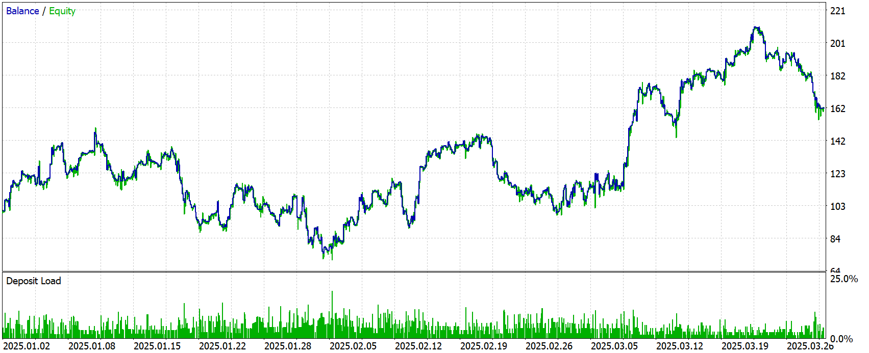
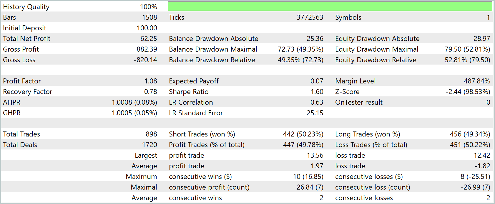
The test results show moderately positive dynamics. Starting with a USD 100 deposit, the EA managed to earn USD 62.25, showing a small positive gap between total profit and total loss. At the same time, the profit factor is barely above 1, which indicates that the strategy is not very effective.
During the testing period, 898 trades were executed, with buy and sell trades split almost evenly. In both cases, the win rate remained around 50%, with a slight bias toward short positions. The average profitable trade yielded USD 1.97, while the average losing trade lost USD 1.82. The maximum profit reached USD 13.56, while the maximum loss was USD 12.42.
Overall, the EA demonstrates stable operation with accurate trade execution, but the strategy's profitability and robustness remain in question.
Conclusion
This article concludes the work on implementing the approaches proposed by the authors of the SSCNN framework using MQL5. The reader has been introduced to the concept of spatiotemporal feature integration, in which each point in time reflects the complex interrelationships between internal data structures and external market impulses.
This model not only broadens our understanding of market behavior, but also provides a tool for adapting to shifts in market regimes — from calm phases to turbulent changes in volatility. The implementation of Attention-based Normalization enhances the focus on significant regions and stabilizes the training process, transforming SSCNN into a flexible analytical mechanism capable of unraveling the structural complexity of financial time series.
References
- Parsimony or Capability? Decomposition Delivers Both in Long-term Time Series Forecasting
- Other articles in this series
Software used in this article
| # | Name | Type | Description |
|---|---|---|---|
| 1 | Study.mq5 | Expert Advisor | Expert Advisor for offline model training |
| 2 | StudyOnline.mq5 | Expert Advisor | Expert Advisor for online model training |
| 3 | Test.mq5 | Expert Advisor | Expert Advisor for model testing |
| 4 | Trajectory.mqh | Class library | Structure for describing the system state and model architecture |
| 5 | NeuroNet.mqh | Class library | Class library for building a neural network |
| 6 | NeuroNet.cl | Library | Code library for an OpenCL program |
Translated from Russian by MetaQuotes Ltd.
Original article: https://www.mql5.com/ru/articles/19134
Warning: All rights to these materials are reserved by MetaQuotes Ltd. Copying or reprinting of these materials in whole or in part is prohibited.
This article was written by a user of the site and reflects their personal views. MetaQuotes Ltd is not responsible for the accuracy of the information presented, nor for any consequences resulting from the use of the solutions, strategies or recommendations described.

 Building a Prop-Firm Compliance Monitor in MQL5 (Part 1): Account Rules and Persistent Settings
 Cricket Algorithm (CA)
 The MQL5 Standard Library Explorer (Part 15): Building a Market-Regime Classifier with dataanalysis.mqh
 A Forgotten Classic in Volume Analysis: The Finite Volume Elements Indicator for Today's Markets

- Free trading apps
- Over 8,000 signals for copying
- Economic news for exploring financial markets
You agree to website policy and terms of use