Forecasting market movements using the Bayesian classification and indicators based on Singular Spectrum Analysis

Introduction

Today, algorithmic trading accounts for about 60-70% of transactions on stock exchanges, and about 90% on FORTS and FOREX markets. Accordingly, the share of robots in the volume of real transactions increases. This is due to the fact that the "Buy And Hold" strategy no longer fits the modern market with active fluctuations in short time intervals. Efficient trade requires a transition from passive investment to active trading. Success in the modern market is based on the use of effective algorithms and a set of system rules that allow increasing the number of successful deals and reduce the number of unsuccessful ones, minimizing the losses.

One promising way to achieve this is building a recommendatory system for time-efficient trading by combining the capabilities of forecasting with the singular spectrum analysis (SSA) and important machine learning method on the basis of Bayes' Theorem. The value of the selected approach lies in that the processing of data is based on the statistical analysis methods exclusively, and does not imply groundless assumptions. This gives a clear idea of both the capabilities and limitations of the method, its perspectives in creating an automated trading system.

During the development of this system, the focus was on the scale of the time frame units from 5 minutes to an hour. A fundamentally larger scale, hours and days, is more popular in the majority of descriptions of theoretically successful statistical methods (due to the reduced contribution of the chaotic component). However, such methods are of little use in the actual practice of individual speculative trading.

Features of application and prediction of price series using SSA

The SSA method is used to solve problems such as:

• separation of the main components of the times series (trend, seasonal variations, oscillation) and noise filtering;
• search for periodicities;
• smoothing of the source data by limiting the set of components;
• prediction of the further behavior of the observed dependence.

SSA is one of the few statistical methods used when working with non-stationary series. Perfect examples of such series are sequences of market prices with their trends, bursts, impulse emissions. At the same time, prices are formed under the influence of independent non-random factors, differing in impact and duration. Assuming that the market depends on such forces most of the time, it is possible to use a model based on the sum of different-scale components, which corresponds to the SSA approach.

Information on the mathematical basis of SSA and its "Caterpillar" version can be found in [1] (see the list of references attached to the article). From a practical point of view, it is important to note that until recently one of the main reasons that influenced the prevalence of SSA in data processing was the absence of fast algorithms similar to FFT. This problem no longer exists — such algorithms have been developed and their effectiveness has been proved [2] (see the list of references attached to the article).

Prediction using SSA uses the model of hidden periodicities: by splitting a data series into components, the behavior of which has been determined during the analysis, it is possible to extend these components according to the behavior parameters and to summarize the result. The outcome is the prediction result, and its quality depends on how well the initial set of components defines the original data. Naturally, the prediction will be unreliable for a chaotically volatile series, but it will be justified for the prices formed under the influence of stable factors and with a relatively small noise. In addition, it is not advisable to rely on statistical analysis when dealing with inactively traded instruments. The impact of individual factors and "major" players in such cases is unpredictable and dangerous.

Combining indicators to increase the reliability of prediction

Three predicting indicators have been developed according to the considered idea. Identification of trend and its prediction - SSA Trend Predictor and Fast Forecast based on the fast transform, SSACD (modification of MACD) and SSA Stochastic. Each indicator is presented in two variants: simplified and extended. 

Since all indicators use the same data, but are aimed at different characteristics of the process, each of them has its advantages and disadvantages. There is a natural desire to combine all the indicators and achieve synergy, increasing the efficiency, robustness and accuracy of evaluating the situation in general.

From the perspective of a speculative strategy, the obvious and demanded information lies in answering the question: "where will the price go in the near future?". There are three options: the price will increase, fluctuate or decrease.

For the indicator that predicts the price according to the identifies trend, it is obvious that the analogue of the derivative must be positive or negative when the price grows or falls. By setting the error level of EPS, a condition can be defined: if the "derivative" is lies in the neighborhood of zero with the radius of epsilon (EPS), then the change in price is negligible.

The SSACD indicator is a modification of MACD, corrected in order to avoid the delay of information, which is commonplace in moving averages. To prevent using too many terms, hereinafter, it will be referred to as MACD. The MACD is displayed on the chart as a histogram and its smoothed exponential moving average, called Signal. Accordingly, the changes in the smoothed line are slightly delayed relative to MACD. Therefore, (MACD-Signal)>0 if the price increases, and (MACD-Signal)<0 if it falls. Setting a certain neighborhood of EPS about the zero, define the transition zone of the unstable price behavior.

The SSA Stochastic indicator is a modified fast Stochastic oscillator with the lag removed, similar to the previous case. Lines of the Stochastic oscillator are typically co-directional to their local trend. That is, the formulation of conditions for the increase, decrease and unstable behavior of the price is possible via the "derivative" of the Stochastic: greater or less than zero, within the epsilon neighborhood.

Since the indicators provide a local forecast, the evaluation of values of the above measurements gives the information on the price behavior in the nearest future. Matching indicator values increase the reliability if the forecast and decrease the possibility of an error.

In order to verify the correctness of the selected approach, it is necessary to evaluate how the combination of indicators allows decreasing the number of critical prediction errors on history data. Errors mean a situation where a short-term prediction indicated one direction, while the price changed in the opposite direction.

Users who have worked with the indicators considered above are probably interested in what control parameter values are selected for them, and why. But since the nearest prediction point is of the most interest, there is no need for a special and long-term selection of these parameters. Suitable parameters for the indicator are the ones that align its behavior with the main (not predictive) part of the series, combining smoothness and detailedness of the price behavior and suitable for a wide class of financial instruments. The following were selected:

1. To predict the price based on trend (SSA Fast Trend Forecast, version 2.5):
   Algorithm: Recurrent forecast,
   N: Data fragment = 256,  
   Time-dependent lag = N/3,
   Trend    high-freq. limit= 0.25,
   Forecast high-freq. limit= 0.25,
   Forecast transform = S[i]/Max(:),
   Forecast smoothing = Smoothing MA(3).
2. For SSACD Forecast (Limited) version 2.5:
   Algorithm: Recurrent forecast,
   N: Data fragment = 512,  
   Time-dependent lag = N/4,
   FastTrend high-freq. limit = 0.4
   SlowTrend high-freq. limit= 0.6
   Signal SMA period = 4
   Data preparation = {ln(S[i]-Smin+1)}/Max(:)
   Forecast preparation = S[i] /Max(:)
   Forecast smoothing = Smoothing MA(3).
3. For SSA Stochastic (Limited) version 2.0:
   Algorithm: Recurrent forecast,
   N: Data fragment = 256,  
   Time-dependent lag = N/4,
   %K high-freq. limit = 0.3,
   %D high-freq. limit = 0.6,
   Data preparation = S[i] /Max(:),
   Forecast smoothing = Smoothing MA(3).

Fragments of historical data for the analysis have been taken at different time intervals:

for GOLD futures on periods M5, M15, H1;

BRENT — M5, M15;

Si-USD/RUB — M15;

for Forex quotes of EUR/USD — M15.

Different trading instruments with different periods were processed with unchanged indicator parameters, which allowed to consider the stability and quality of the forecast values. Iteration over the data series of length about 1000 points with calculation of the forecast at each point in history provided an opportunity to compare the forecasts and facts.

Let us illustrate the results of the indicators' predictions based on the Close price data on the charts.

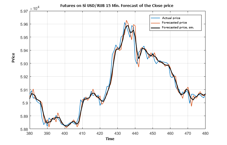
Figure 1. Fragment of comparison of the actual Close price, its predicted value and prediction value smoothed by three points

Fig. 1 shows that prediction "by trend" is slightly delayed most of the time. This is not surprising, since the trend-based price prediction is set for versatility of application for different financial instruments and it is smooth because a significant part of high-frequency oscillations is filtered out. A similar behavior of the forecast takes place for other instruments (BRENT, GOLD) at different time frames (5 minutes and 1 hour).

Let us compare a prediction of another indicator evaluation (MACD-Signal) with its actual value.

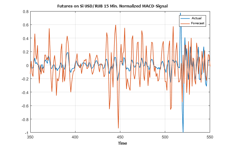
Figure 2. Fragment of the actual and forecast values of the price evolution direction according to the MACD indicator 

Figure 3. Consistency of the formed trend in the price changes and prediction of the price changes according to MACD

The border of direction uncertainty (EPS) was set to 0.25 from the standard of the normalized (by the maximum amplitude) of the series values (MACD-Signal).

A fragment of the comparison of the stochastic and the preliminary forecast formed at each point with the help of the "SSA Stochastic" indicator is shown in the following figure.

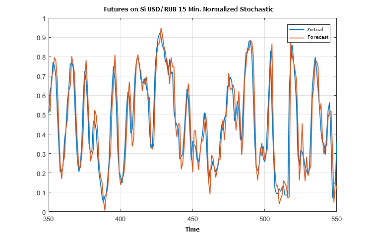
Figure 4. Actual and forecast values for Stochastic 

Figures 2 and 4 illustrate almost a complete equiphase condition of the predictions and actual outcome according to the data of the SSACD and SSA Stochastic indicators. This can probably be expected when applying the SSA prediction for many oscillators.

Since the price predictions presented in the Figure 1 contain a set of errors in direction, let us find out how a combination of the indicators allows reducing the number of such errors. The difference in the values of the actual and predicted price in Figure 1 is irrelevant, because it does not cause losses when in a concordant position. 

There are values: (MACD-Signal), difference derivatives for series of the actual and predicted price and stochastic, smoothed by three points. The consistency of the conditions defined earlier, which indicate the direction of the price change, is further used to analyze the efficiency of their combination. 

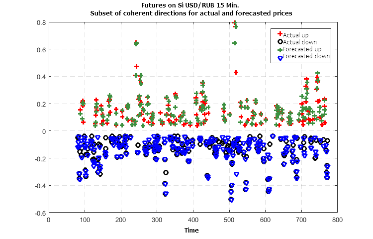
Figure 5. Concurrency of the actual and predicted directions of the changes in price when using three indicators

 

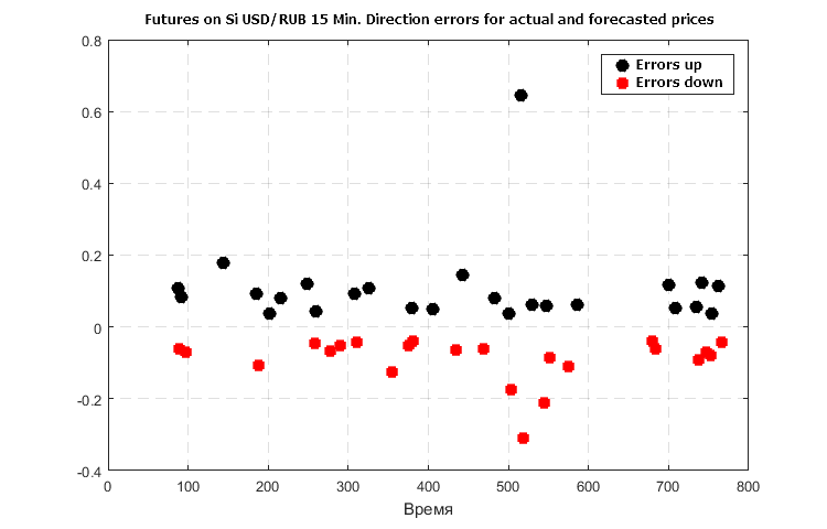
Figure 6. Considerable errors in forecast of the price change direction in case only the trend-based prediction is used

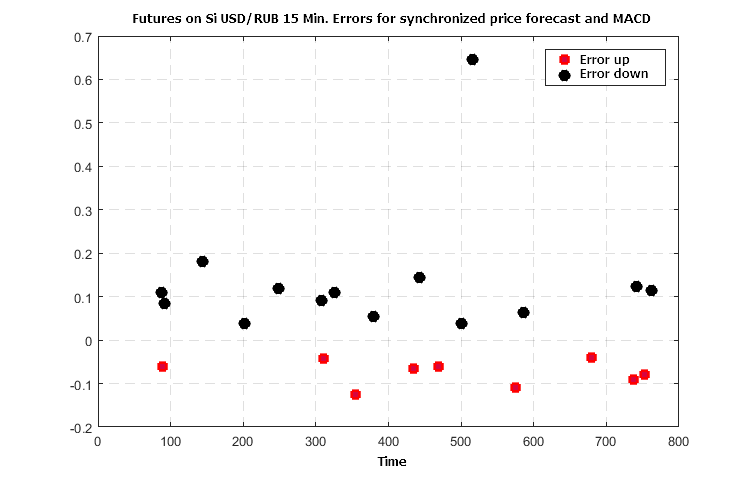
Figure 7. Error in forecast for a combination of price predictions based on trend and (MACD-Signal)

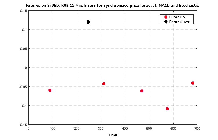
Figure 8. Error in forecast for a combination of price predictions based on trend, MACD and Stochastic

Figures 6 — 8 demonstrate a synergistic effect of the use of three indicators — the number of crude errors in forecasting the direction of the further price changes falls no worse than 5 to 7 times with the agreed values of the indicator functions. 

Bayes classifier of probable price movements based on forecast values of indicators

The Bayes' theorem is presented in the basic course of probability theory and relates the conditional probability of event x provided that the event y had taken place.

By definition:  ,  where is the joint probability of x and y, while p(x) and p(y) are the individual probabilities of each event. Accordingly, the joint probability can be expressed in two ways:

Bayes' theorem:

 

For the considered situation with the forecast of the price movement direction based on indicators, the theorem can be rewritten in the following form:

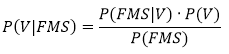
where:

V — event that corresponds to the actual price movement in a given direction (sign of its change). Three possible options: V1= -1 "down", V2 = 0 "uncertain", V3 = +1 "up".

F — event corresponding to the forecast of the price direction or the sign of the predicted derivative (three possible options: F1 = -1 "down", F2 = 0 "uncertain", F3 = +1 "up").

M — event corresponding to the forecast of the (MACD-Signal) sign, consistent with the price behavior (three possible options: M1 = -1 "down", M2 = 0 "uncertain", M3 = +1 "up").

S — event corresponding to the sign of the predicted Stochastic derivative (three possible options: S1 = -1 "down", S2 = 0 "uncertain", S3 = +1 "up").

The left part of the formula can be translated to a human-readable form as follows: "What is the probability of price moving in the direction Vk={-1,0,1}, if the forecast indicators give specific values ​​of F, M, S?".

Next, in order to simplify the presentation, we will say that the indicators take the values of -1, 0, +1, implying the sign of the derivative or the sign of (MACD-Signal). 

To evaluate and compare the probabilities of whether the price goes down, up or remains weakly fluctuating, it is necessary to know the values on the right side of the formula. To do this, two tasks will be solved:

1. perform "learning" on history data,
2. study the "stability" of the learning results on data outside the training interval.

Variants of training have been performed in different data fragments, on different timeframes and instruments. The training sample had a length of several hundred bars. The results turned out to be similar, as would be expected due to the universality of the selected parameters of the indicators considered in the third section of the article.

Let us illustrate the results on the analysis of the "Close" price data of the futures on USD/RUB 15 M. 

We restrict ourselves to studying the probability of the price going "up" and "down", as those two values are used as the basis for making a decision on opening or closing a deal.

It is quite understandable that in case of a real downward movement of the price, the indicator signals must also be negative ("down") or close to zero ("neutral"). This is confirmed by the first evaluation of the conditional probabilities of joint forecast events when the price falls. However, other probabilities, obtained from the results of training on the data of USD/RUB-15M futures, indicate the possibility of deviations from expected values, which is presented in Tables 1, 2.

Results of calculations based on the Bayes' formula give an interesting information of distribution of the real movement probability depending on the indicator values. The maximum conditional probabilities of the prices going down (event V1 =-1) and up (event V3 = +1) depending on the predicted values are presented in tables 3 and 4.

The classification levels will be simple: if the conditional probability of a "downward movement" event is greater than 0.5 at the current moment and at the same time it is greater than the probability of an "upward" movement, the movement forecast is down. The condition for an "upward" movement of the price is similar.

Here is the result of training in the form of a price chart with the classification marks.

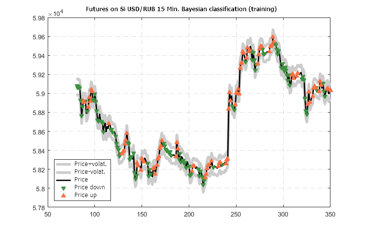
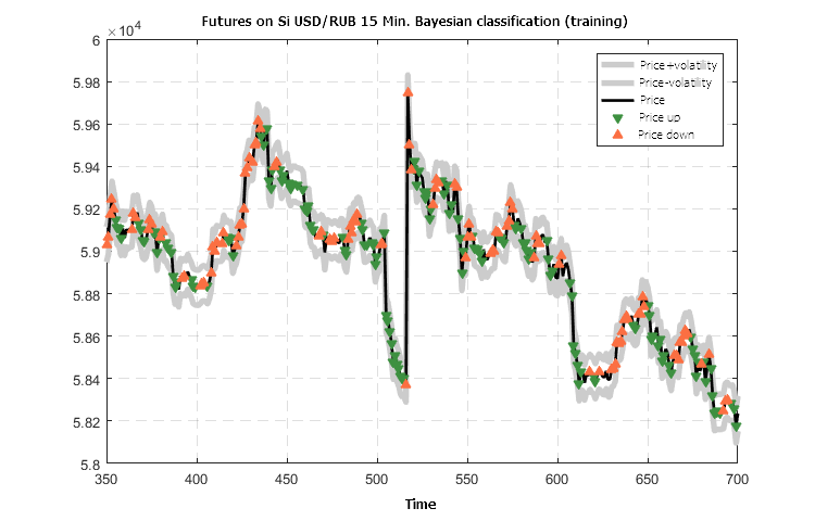
Figure 9. Predicted classification of the USD/RUB-15 futures price movement calculated based on training data 

The classification results presented in Figure 9 look noteworthy: forecasting of the direction for the nearest future manages to quickly switch the movement direction pointer and maintain it. 

The main question remains to be examined: robustness of the training results presented by a matrix of conditional probabilities P(V|FMS), so that they can be propagated to an external situation (relative to the training data).

Historical series of other financial instruments on other timeframes will be taken to check the robustness. With the forecast values of indicators known for each individual moment of time, perform a classification by direction, using the prepared matrix of conditional probabilities calculated for the futures on USD/RUB-M15. Compare the classification result with the actual situation.

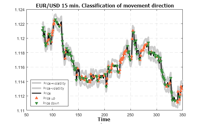
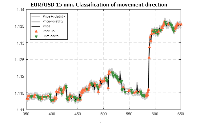
Figure 10. Predicted classification of the EUR/USD-15M quotes movement (trained on the USD/RUB-15M futures)

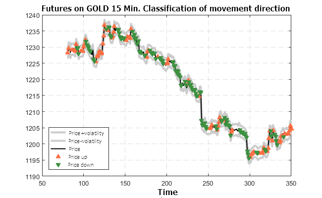
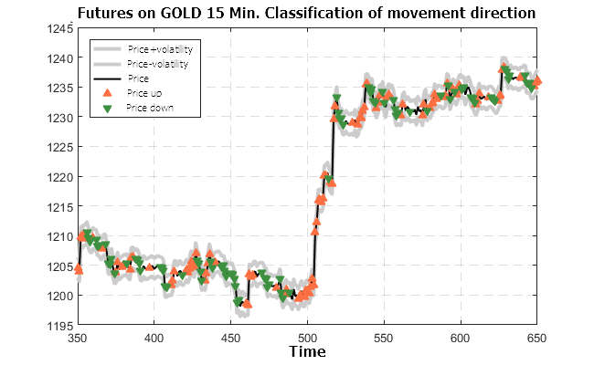
Figure 11. Predicted classification for the futures on GOLD-15M (trained on the USD/RUB-15M futures)

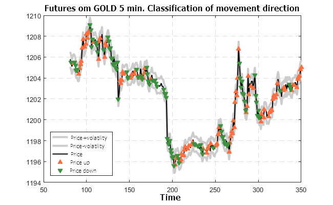
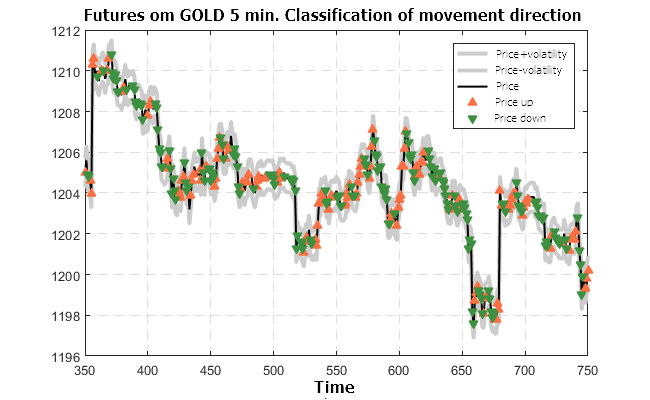
Figure 12. Predicted classification for the futures on GOLD-5M (trained on the USD/RUB-15M futures)

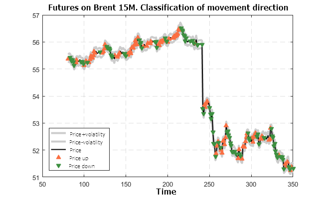
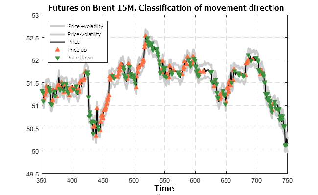
Figure 13. Predicted classification for the futures on BRENT-5M (trained on the USD/RUB-15M futures)

The results shown in Figures 10 — 13 look very optimistic. The classifier prepared using the futures on USD/RUB-15M is valid for other timeframes and other financial instruments.

Recommended system based on the Bayesian classifier

The presented classifier can be used as a basis for designing a constructive recommendatory system, and then a trading system with few control parameters. A limited number of parameters allows for effective optimization.

In order not to be unfounded, let us consider the application of the system on historical data. Of course, the result has a remote relation to the real situation, since everything is fundamentally simplified, but it shows the potential laid in the system.

There are 4 main control parameters:

1. Risk Ratio — stop level as a multiple of volatility.
2. Risk Fix     — allowable fluctuation in the opposite direction when opening a trade and keeping a profitable position (as a multiple of volatility).
3. Probability Trade Min — allowable probability for keeping a trade.
4. Probability Trade OK — the probability, at which taking a trade is recommended.

In this case, the volatility will be measured by the root mean square average of the difference between the opening and closing prices on the fragment of the processed data. The stop level is tied to the previous Close prices and it is shifted in one direction. Decision to enter and exit a position is taken after a bar is closed.

The recommendations of the system trained on the data of the USD/RUB-15M futures were used to simulate trading the GOLD-15M futures individually according to the history of Close prices shown in Figure 11 and prediction classification controlled by the control parameters 3 and 4. The charts below show the change in the profitability depending on "time", measured in the number of bars.

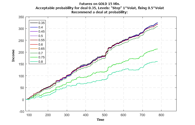
Figure 14. Influence of the probability value of the deal recommendation on the profitability of trading the GOLD-15M futures individually (trained on the USD/RUB-15M futures)

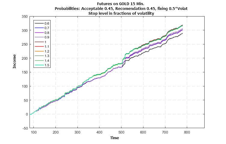
Figure 15. Influence of the stop level parameter on the profitability of trading the GOLD-15M futures individually (trained on the USD/RUB-15M futures)

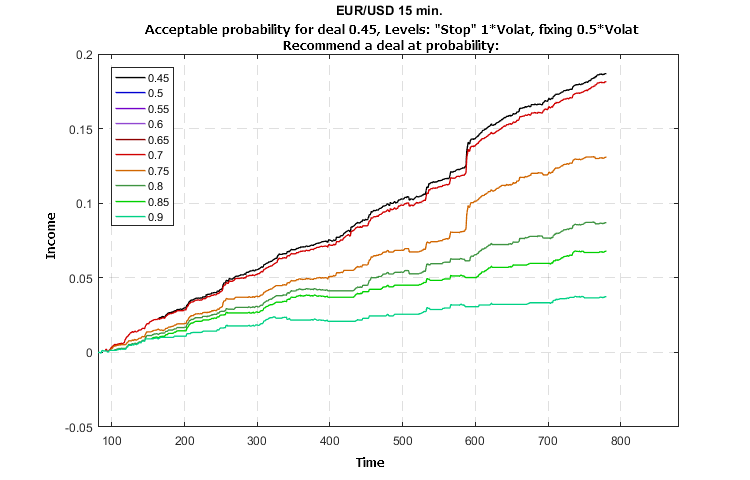
Figure 16. Influence of the probability value of the deal recommendation on the profitability of trading the EUR/USD-15M quotes individually (trained on the USD/RUB-15M futures)

The simulation results shown in Figures 14 — 16 indicate a stable growth in profitability without major losses. The influence of the parameter values on the growth of profitability indicates the possibility and efficiency of optimization. 

Program for rapid assessment of market dynamics

The next work describes the structure, rules and testing results of an automated trading system. However, it will be logical to provide a software module designed for rapid assessment of the situation and "recommendations" during live trading. The work comes with a module that solves the classification problem and works with different indicator pairs: a) SSACD Forecast Limited and SSA Stochastic Limited, b) SSACD Forecast and SSA Stochastic. SSACD must be at least version 2.5, and Stochastic — at least 2.0. In case the full versions of the indicators are used, the program allows for a better customization of the classification control parameters and provides the options of training on different data, which makes it possible to select the "closest" model prepared for the forecast classification. Forecast "by trend" is performed within the module, therefore, a separate instance of the SSA Fast Trend Forecast indicator is not required.

It should be noted, however, that the program uses the incorporated model and therefore does not guarantee, but rather helps evaluate the development of the price for actively traded instruments. One should not rely on statistical forecast of the price for a situation with a small number of deals, as individual stimuli may have too much of an impact. The same applies to time intervals or periods when the price has a "gap"-like behavior.

The Expert Advisor is called SSA Bayes Observer. At startup, it offers to set the values of parameters considered above.

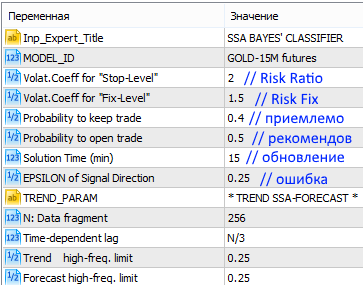
Figure 17. Starting the SSA Bayes Observer program with the default parameters

In addition to the main values of Observer, it is also possible to set the parameters for the trend-based forecast indicator, SSACD and SSA Stochastic. Their meaning and purpose have been discussed in the descriptions of the indicators themselves, but it possible to rely on the preset default values.

If the SSACD and SSA Stochastic indicators of the latest version are installed in the system, user will see an interface similar to the following:

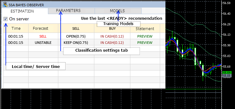
Figure 18. Interface of the SSA Bayes Observer program

The current settings can be changed while the program is running, by selecting the corresponding tab.

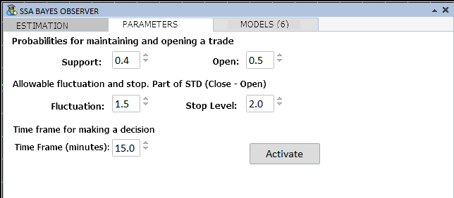
Figure 19. Classification parameters 

The model to be used as the basis for classification can be selected on the MODELS tab:

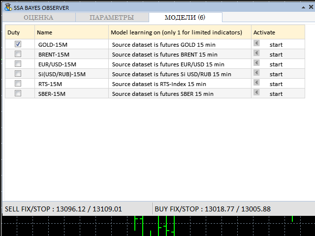
Figure 20. Tab for selecting the training model

The control parameters shown in Figures 18 — 20 can be adjusted while the program is running. Training models can be selected only if the full versions of the SSACD and SSA Stochastic indicators are available.

During the operation, the program has an interface similar to the following:

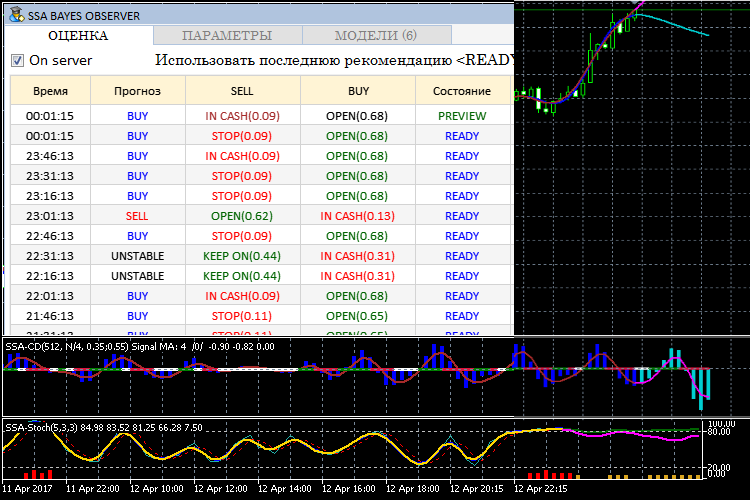
Figure 21. Operating mode of SSA Bayes Observer 

As it can be seen in Figure 20, the lower line of the interface windows shows FIX and STOP — levels for different trading modes. They serve to exit positions if the price exceeds them. The FIX level is designed for situations when the deal developed successfully. The STOP level implies an unconditional closure of a position. It is assumed that the decision on exiting the position is taken after the analyzed time interval is completed (the READY label).

Conclusion

This work presents the methodology and algorithm of building a recommendatory system for time-efficient trading by combining the capabilities of forecasting with the singular spectrum analysis (SSA) and important machine learning method on the basis of Bayes' Theorem. Modeling has been carried out in order to determine the feasibility of applying a system trained on a set of certain data to the analysis of time series of another time frame and other financial instruments. A program has been presented, which allows considering the feasibility of the method's application to the analysis of real data in practice. Description of the program's structure and explanation of the code will be provided in the next article.

The practical application of the classification in real time has revealed a number of problems, which must be solved in order to formulate a strategy suitable for automation of trading. They will also be discussed in the next part of the work.

I want to express special gratitude to Anatoli Kazharski for the development of the graphical interface [3], the use of which has delivered from hard and time-consuming work, as well as to specialists, who have provided the MQL implementation of the excellent mathematical library ALGLIB [4].

List of References

1. N. E. Golyandina The "Caterpillar"-SSA method: forecast of time series. Study Guide. Saint-Petersburg, 2004.
2. Korobeynikov, A. Computation- and space-efficient implementation of SSA. // Statistics and Its Interface. 3, 2010, 3, 357-368.
3. https://www.mql5.com/en/articles/3173
   
4. https://www.mql5.com/en/code/1146