Stress Testing Trade Sequences with Monte Carlo in MQL5

• Introduction
• Method
• Implementation
  • Input Parameters and Global Variables
  • Loading Trade Data
  • Bootstrap Simulation Engine
  • Metrics Computation
  • Chart Rendering
  • CSV Export
• How to Use the Script
  • Preparing the trades.csv File
  • Running the Script
• Results
• Interpretation
• Limitations
• Extensions

Introduction

A backtest ending with 42% net profit and a 1.8 profit factor looks great on paper. But here's the uncomfortable truth: that result is path-dependent. The specific sequence of wins and losses in your historical data produced that particular equity curve—and if the same trades had arrived in a different order, the outcome could've been dramatically different.

We watched this happen firsthand with a trend-following EA on EURUSD M30. The strategy had a positive expectancy, a decent win rate, and a profit factor just above 1.6. Looked fine. But when we ran it through a sequence stress test, we found that roughly 12% of alternative trade orderings would have triggered a margin call before reaching trade 80—out of a 200-trade history. Same trades. Same edge. Just different luck on the order. That's the problem nobody talks about at the backtest stage.

And it's worse than it sounds. A trader looking at a single equity curve has no way of knowing whether the strategy is genuinely robust or just got lucky with the sequence. Honestly, most traders stop there—one backtest, looks good, go live. That's a mistake we've seen end badly more than once.

Quantitative risk managers addressed this decades ago with Monte Carlo simulation. They generate thousands of "what-if" scenarios from the same data to reveal the distribution of outcomes, not just a single historical path. In trading terms, given N trades and their realized P&L, what if the same trades occurred in a different order? Critically, how often would the strategy breach a catastrophic drawdown threshold before the sample ends?

MonteCarlo_RiskAssessor.mq5 reads trade P&L from a CSV file and runs 1000 bootstrap simulations. It renders a multi-percentile fan chart directly in MetaTrader via CCanvas and exports percentile curves to a machine-readable output file. Commission and slippage can be layered in to stress test results under realistic execution conditions. No external libraries needed.

Method

Here's the core idea: bootstrap resampling—the simplest, most assumption-free form of Monte Carlo available.

Given a set of historical trade outcomes (P&L values), we treat each trade as an independent observation drawn from some unknown distribution. For each simulation run, we draw N trades at random with replacement from the historical pool, then accumulate them into a synthetic equity curve starting from the initial balance. Repeat 1000 times, and we have 1000 plausible equity paths. Not predictions of the future. A realistic exploration of how volatile the path could've been, even with the same underlying edge.

Why bootstrap instead of a parametric model (e.g., fitting a normal distribution)? Because real P&L distributions are not normal. They're fat-tailed, often skewed, and sometimes bimodal. A mean-reversion strategy running on GOLD H1 might have a return distribution that looks nothing like a bell curve—it'll have a cluster of small wins, a few large losses, and maybe a fat right tail from the occasional big trending day caught perfectly. Fitting a normal to that and sampling from it smooths out exactly the outliers that matter most for drawdown estimation. Bootstrap doesn't assume anything about the shape. It samples from what actually happened.

The five percentile curves—5th, 25th, 50th, 75th, and 95th—form the fan chart that anchors the output. The 50th percentile is the typical outcome. The 5th percentile is the "rough run" scenario: 95% of simulations ended above this level. The width of the fan at any given trade step is a direct visual measure of outcome uncertainty. A wide fan early in the series means the strategy is sensitive to sequence effects. That's worth knowing before you go live.

Four core risk metrics come out of the full simulation set. Median Max Drawdown—the typical worst peak-to-trough decline. Stress Drawdown (95th percentile)—the drawdown exceeded in only 5% of runs: a stress-test figure, not a floor. Value at Risk (5%)—the dollar amount at risk at the 5th percentile of final equity, computed as Initial Balance − P5_Final_Equity. And probability of ruin—the fraction of simulations where max drawdown exceeded the configured ruin threshold (set to 20% in our test run).

The slippage simulation (Feature #3) adds a per-trade cost drawn from [0, InpSlippageMax] plus a fixed commission, deducted from every sampled trade regardless of direction. Worst-side fill assumed throughout—conservative, but that's the point.

Implementation

Input Parameters and Global Variables

Worth noting before we dive in: this is a script, not an EA. It runs once on demand—no tick-by-tick loop, no persistent state between runs. Everything gets computed in a single OnStart() call.

The input block exposes all configurable parameters without requiring code edits. Below are the declarations, along with the global arrays that carry data between function calls:

//--- Core simulation inputs
input string   InpCSVFile         = "trades.csv";    // CSV file in MQL5\Files\
input int      InpSimulations     = 1000;             // Number of MC simulations
input double   InpInitialBalance  = 10000.0;          // Starting account balance ($)
input double   InpRuinThreshold   = 0.20;             // Ruin = 20% drawdown
//--- Feature #3: Commission & slippage stress-test
input bool     InpSlippageEnabled = false;
input double   InpCommission      = 2;                // Fixed commission per trade ($)
input double   InpSlippageMax     = 3;                // Max random slippage per trade ($)
//--- Feature #2: CSV export
input bool     InpExportCSV       = true;
input string   InpExportFile      = "mc_results.csv";
//--- Global data arrays
double g_Profits[];         // Trade P&L values from CSV
double g_FinalEquities[];   // Final equity per simulation
double g_MaxDrawdowns[];    // Max drawdown (%) per simulation
double g_AllCurves[];       // Flattened [sim × (tradeCount+1)] equity matrix
int    g_TradeCount = 0;
//--- Shared summary metrics
double g_p05Eq, g_p50Eq, g_p95Eq;
double g_p50DD, g_p95DD;
double g_varAmt, g_probRuin;

The array g_AllCurves[] is the critical data structure. It's a flattened 2D matrix storing the complete equity path for every simulation. Flat storage—rather than a jagged array—makes row access fast: sim * curveLen + step. When the rendering pass iterates over hundreds of trade steps, drawing five percentile lines, that index arithmetic saves a noticeable amount of time on larger datasets.

Loading Trade Data

LoadTradesFromCSV() handles CSV ingestion with tolerance for both single-column (P&L only) and two-column (date, P&L) formats. Here's the full function:

//+------------------------------------------------------------------+
//| Load trade P&L from CSV into g_Profits[]                         |
//+------------------------------------------------------------------+
bool LoadTradesFromCSV(const string fileName)
  {
   int handle = FileOpen(fileName, FILE_READ | FILE_CSV | FILE_ANSI, ',');
   if(handle == INVALID_HANDLE)
     {
      PrintFormat("ERROR: Cannot open '%s'. Verify file is in MQL5\\Files\\. Code: %d",
                  fileName, GetLastError());
      return false;
     }
   if(!FileIsEnding(handle))
      FileReadString(handle);  // skip header row
   double buffer[];
   int    count = 0;
   while(!FileIsEnding(handle))
     {
      string row = FileReadString(handle);
      StringTrimRight(row);
      StringTrimLeft(row);
      if(StringLen(row) == 0) continue;
      string cols[];
      int nCols = StringSplit(row, ',', cols);
      double profit = 0.0;
      if(nCols >= 2)
         profit = StringToDouble(cols[1]);
      else if(nCols == 1)
         profit = StringToDouble(cols[0]);
      ArrayResize(buffer, count + 1, 1000);
      buffer[count++] = profit;
     }
   FileClose(handle);
   if(count == 0) { Print("ERROR: No valid trade data found."); return false; }
   ArrayResize(g_Profits, count);
   ArrayCopy(g_Profits, buffer, 0, 0, count);
   g_TradeCount = count;
   return true;
  }

The ArrayResize(..., 1000) call pre-allocates memory in chunks of 1000 during the read loop—this avoids the cost of per-element reallocation on large histories. Practical note: Strategy Tester CSV exports often place the profit column at index 12 rather than index 1. A one-line change to target cols[12] is all it takes. We've had to do that more than once when switching between export formats.

Bootstrap Simulation Engine

This is where the real work happens. RunMonteCarloSimulation() runs N independent simulations, each one randomly sampling from the trade pool with replacement and accumulating an equity path. Slippage and commission get deducted per trade when enabled:

//+------------------------------------------------------------------+
//| Bootstrap Monte Carlo engine                                      |
//| Feature #3: optionally subtract commission + random slippage     |
//+------------------------------------------------------------------+
void RunMonteCarloSimulation()
  {
   int curveLen = g_TradeCount + 1;
   ArrayResize(g_FinalEquities, InpSimulations);
   ArrayResize(g_MaxDrawdowns,  InpSimulations);
   ArrayResize(g_AllCurves,     InpSimulations * curveLen);
   double equity[];
   ArrayResize(equity, curveLen);
   MathSrand((int)TimeLocal());
   for(int sim = 0; sim < InpSimulations; sim++)
     {
      equity[0] = InpInitialBalance;
      for(int t = 0; t < g_TradeCount; t++)
        {
         int    rIdx = MathRand() % g_TradeCount;
         double pnl  = g_Profits[rIdx];
         //--- Feature #3: apply fixed commission + uniform-random slippage
         if(InpSlippageEnabled)
           {
            double slip = ((double)MathRand() / 32767.0) * InpSlippageMax;
            pnl -= (InpCommission + slip);
           }
         equity[t+1] = equity[t] + pnl;
        }
      g_FinalEquities[sim] = equity[g_TradeCount];
      g_MaxDrawdowns[sim]  = CalcMaxDrawdown(equity, curveLen);
      //--- Store full curve in flattened matrix
      ArrayCopy(g_AllCurves, equity, sim * curveLen, 0, curveLen);
     }
  }

The slippage model is intentionally conservative: both the fixed commission and a random draw from [0, InpSlippageMax] are deducted from every trade, regardless of direction. Worst-side fills are assumed throughout. On GOLD with strategies holding positions for less than 4 hours, we've found this conservative framing lines up reasonably well with live execution costs—at least in our testing on ECN accounts with typical spreads of 1.5–2 pips.

CalcMaxDrawdown() scans forward through each equity path, tracking the running peak:

//+------------------------------------------------------------------+
//| Calculate peak-to-trough max drawdown (returns %)               |
//+------------------------------------------------------------------+
double CalcMaxDrawdown(const double &eq[], int len)
  {
   double peak  = eq[0];
   double maxDD = 0.0;
   for(int i = 1; i < len; i++)
     {
      if(eq[i] > peak) peak = eq[i];
      if(peak > 0.0)
        {
         double dd = (peak - eq[i]) / peak;
         if(dd > maxDD) maxDD = dd;
        }
     }
   return maxDD * 100.0;  // return as percentage
  }

Metrics Computation

ComputeMetrics() collapses the full simulation dataset down to seven numbers. The Percentile() helper uses linear interpolation on a sorted copy—the same method as NumPy's percentile and Excel's PERCENTILE.INC, so results are directly comparable if you export to Python or a spreadsheet:

//+------------------------------------------------------------------+
//| Percentile helper (linear interpolation on sorted copy)          |
//+------------------------------------------------------------------+
double Percentile(double &arr[], double pct)
  {
   int n = ArraySize(arr);
   if(n == 0) return 0.0;
   double tmp[];
   ArrayCopy(tmp, arr);
   ArraySort(tmp);
   double pos = pct * (n - 1);
   int    lo  = (int)MathFloor(pos);
   int    hi  = (int)MathCeil(pos);
   if(lo == hi) return tmp[lo];
   return tmp[lo] + (tmp[hi] - tmp[lo]) * (pos - lo);
  }
//+------------------------------------------------------------------+
//| Compute and cache all summary metrics into globals               |
//+------------------------------------------------------------------+
void ComputeMetrics()
  {
   g_p05Eq   = Percentile(g_FinalEquities, 0.05);
   g_p50Eq   = Percentile(g_FinalEquities, 0.50);
   g_p95Eq   = Percentile(g_FinalEquities, 0.95);
   g_p50DD   = Percentile(g_MaxDrawdowns,  0.50);
   g_p95DD   = Percentile(g_MaxDrawdowns,  0.95);
   g_varAmt  = InpInitialBalance - g_p05Eq;
   int ruinCount = 0;
   for(int i = 0; i < InpSimulations; i++)
      if(g_MaxDrawdowns[i] >= InpRuinThreshold * 100.0)
         ruinCount++;
   g_probRuin = (double)ruinCount / InpSimulations * 100.0;
  }

Results get cached in globals so both DrawResultsOnChart() and ExportResultsToCSV() can read them without recomputing. PctAtStep() is a companion function that extracts the cross-sectional percentile at a specific trade step—gathering one value from every simulation's stored curve, then calling Percentile() on that slice. It's the engine behind the fan chart.

Chart Rendering

DrawResultsOnChart() builds the visual output using CCanvas—MetaTrader's built-in bitmap canvas. There are seven rendering layers drawn in sequence: filled percentile bands, percentile boundary lines, right-side inline labels, reference line and grid, title, legend, and the stats panel.

The Y-axis scale comes from the 5th–95th envelope across all trade steps. This ensures the fan always fills the chart area, even when the outcome spread is wide:

//--- Y-scale: 5th–95th envelope across all steps
double yMin = DBL_MAX, yMax = -DBL_MAX;
for(int s = 0; s <= g_TradeCount; s++)
  {
   double lo = PctAtStep(s, 0.05);
   double hi = PctAtStep(s, 0.95);
   if(lo < yMin) yMin = lo;
   if(hi > yMax) yMax = hi;
  }
double yRange = (yMax > yMin) ? yMax - yMin : 1.0;

Two macros handle the data-to-pixel conversion:

#define XP(step) (cL + (int)((double)(step) / g_TradeCount * cW))
#define YP(val)  (cB - (int)(((val) - yMin) / yRange * cH))

The inner and outer bands use FillTriangle() with alpha-blended colors: 45 alpha for the wide 5th–95th band and 110 for the tighter interquartile 25th–75th band. The median curve gets a 3-pixel weight. Implementation detail: the right-side inline labels use a two-pass collision-avoidance algorithm. The first pass pushes labels forward to enforce a minimum gap; the second pulls them back to reduce crowding. Without it, labels stack on top of each other whenever percentile curves converge at the series endpoint.

CSV Export

ExportResultsToCSV() writes a three-section output file: a metadata header, a step-by-step percentile table (one row per trade, five percentile columns), and a summary metrics block. The file is written in FILE_ANSI mode for broad compatibility with spreadsheet tools.

//--- Section 2: percentile curves—one row per trade step
FileWriteString(h, "Step,P5_Equity,P25_Equity,P50_Equity,P75_Equity,P95_Equity\n");
for(int s = 0; s <= g_TradeCount; s++)
  {
   FileWriteString(h, StringFormat("%d,%.2f,%.2f,%.2f,%.2f,%.2f\n",
                   s,
                   PctAtStep(s, 0.05),
                   PctAtStep(s, 0.25),
                   PctAtStep(s, 0.50),
                   PctAtStep(s, 0.75),
                   PctAtStep(s, 0.95)));
  }

The exported file can be used in Excel or Python. Typical uses include plotting percentile curves (matplotlib), fitting distributions to final equity, and computing rolling Sharpe ratios across simulated paths. In practice, we load the mc_results.csv into a pandas DataFrame and run a quick seaborn lineplot on the percentile columns—it takes about three lines of Python and produces a publication-ready chart, not necessary for MQL5 use but useful for reporting.

How to Use the Script

Before looking at results, it helps to know exactly how to get the script running—and where the input data comes from. This section covers both.

Preparing the trades.csv File

The script reads trade P&L values from a CSV file placed in the MQL5\Files\ directory. There are two ways to generate this file.

Option 1—Export from MetaTrader Strategy Tester (recommended). This is the most common workflow. After running a backtest, open the Strategy Tester panel, navigate to the Results tab, right-click anywhere on the trade list, and select "Save as Report." The exported file will contain one row per closed trade with multiple columns. The profit column is typically at index 12 in a full Strategy Tester export—in that case, open the file and either delete the other columns, leaving only the profit values, or adjust the LoadTradesFromCSV() function to target cols[12] directly.

The script only needs the profit column—no date, no ticket number, nothing else. The expected format is a single-column CSV:

Profit
125.40
-87.20
203.75
...

A header row is optional. The loader skips it automatically if present.

Option 2—Build manually from any trade log. If your trade history comes from a live account, a third-party platform, or a spreadsheet, copy the closed-trade profit column into a plain text file—one value per row, positive for wins, negative for losses. Save it as trades.csv (or any name—configurable in the script inputs). That's it.

Running the Script

Once the CSV is ready, the workflow is three steps.

Step 1—Place the file in the correct folder. Copy your trades.csv to MQL5\Files\ on your machine. In MetaTrader 5, this folder is accessible via File → Open Data Folder → MQL5 → Files. The script can only read files from this directory.

Step 2—Attach the script to any chart. Drag MonteCarlo_RiskAssessor from the Navigator panel onto any open chart—the symbol and timeframe don't matter, since the script reads from a file rather than live market data. An input dialog will appear.

Step 3—Configure the settings and click OK. The default settings are a reasonable starting point for most strategies.

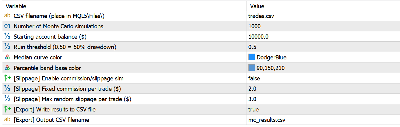
Figure 1: Script input dialog in MetaTrader 5—default settings

Click OK. The script runs in a few seconds for 1000 simulations on a typical trade history. The fan chart panel appears on the chart, and if InpExportCSV is enabled, mc_results.csv is written to MQL5\Files\ automatically.

One thing worth knowing: the script renders the panel as a bitmap label object. If the chart is closed and reopened, the panel won't persist—just run the script again. It takes under 10 seconds.

Results

The script was tested on a trade history exported from MetaTrader's Strategy Tester—a trend-following EA on GOLD H1 covering 182 closed trades from January to April 2026. Initial balance set to $10,000, simulations to 1000, ruin threshold at 20% drawdown. Slippage simulation was disabled for this run.

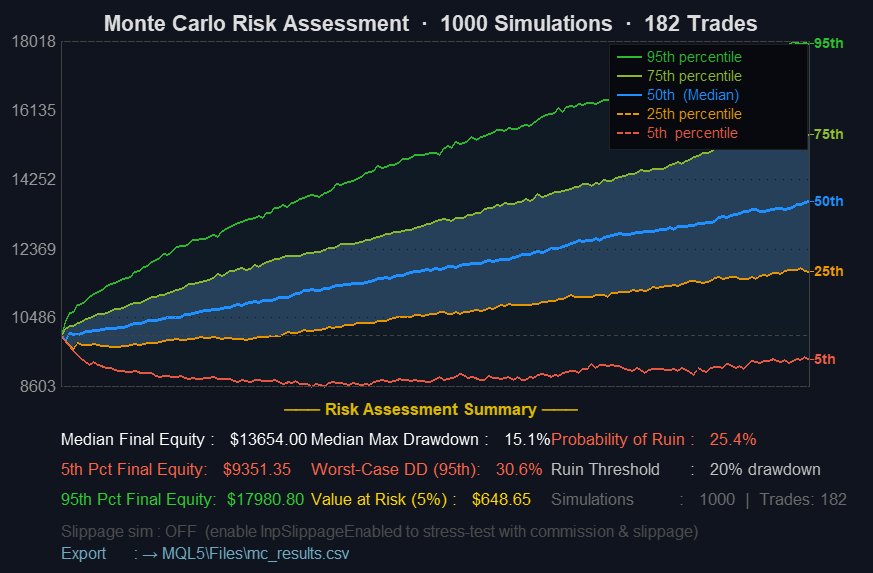
Figure 2: Full Monte Carlo fan chart output—1000 simulations, GOLD H1

The statistics panel reported the following:

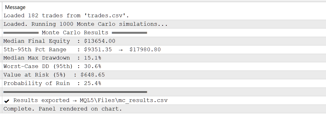
Figure 3: MetaTrader 5 Expert Log Output

Interpretation

The fan chart is where most of the analytical value lives—and it's worth spending time reading it properly rather than jumping straight to the probability-of-ruin number.

The width of the fan at any given trade step is the primary signal. A narrow fan means that regardless of sequence, outcomes converge—the edge is consistent enough that path dependency matters less. A wide fan, especially one that diverges quickly in the first 30–40 trades, is a warning: the strategy's outcome is highly sensitive to trade order. That can mean a run of early losses is dangerous even when the overall expectancy is positive. We've seen accounts blow up during the first 60 trades of a 200-trade system that had a perfectly acceptable final equity in the historical backtest. The fan would've shown it.

The slope of the median curve relative to the initial balance line tells you about expected drift. In our test run, the median curve climbs from $10,000 to $13,654.00 across 182 trades—a 36.5% gain in the typical scenario. That's a clear positive slope, confirming that the edge holds in the majority of simulated paths. If the median barely clears the starting balance, the edge is thin—maybe too thin to absorb real execution costs that weren't modeled.

Does a probability of ruin at 25.4% mean the strategy is unsafe? It depends on how you read it. It means that in nearly 1 in 4 simulated trade sequences, the drawdown hit the 20% ruin threshold at some point. The tool highlights this in red for a reason—and honestly, 25.4% is worth taking seriously before going live. Under the assumptions of this simulation—i.i.d. trades, fixed lot sizes, no regime shifts—that figure suggests the strategy has meaningful sensitivity to trade ordering, especially in its early trades. That's a useful signal, not a verdict.

Value at Risk translates the 5th percentile outcome into a dollar figure. Here it's $648.65—meaning in the worst 5% of simulated paths, the account loses at least $648.65 from the $10,000 starting balance. On a $10,000 account, that's manageable. But scale the lot size up 3×, and that same VaR becomes $1946—a number that starts to feel less comfortable. This feeds directly into position sizing decisions. If the VaR figure is uncomfortable relative to account size, the fix is proportional lot size reduction—not strategy replacement.

The Stress Drawdown (95th percentile) is the number to anchor risk planning around. Here it lands at 30.6%—double the median max drawdown of 15.1%. In our testing across several trend-following systems—on GOLD, EURUSD, and NAS100 H1—the 95th percentile MC drawdown tends to be 1.5–2.5× the drawdown seen in the original backtest sequence. At 30.6%, this result sits squarely in that range. If the live account can't absorb that drawdown, the strategy is over leveraged for the account size. And that's the key insight the single backtest never gives you.

Limitations

Bootstrap MC isn't a crystal ball. There are real structural constraints, and we're not hiding them.

The biggest gotcha: trade independence. Bootstrap resampling treats each trade as an independent draw. No serial correlation is modeled between consecutive outcomes. In reality, many strategies produce correlated results—winning streaks and losing streaks cluster because they reflect underlying market conditions. A trend-follower struggling during a choppy range will produce a run of losing trades that aren't independent at all. Bootstrap spreads those losses randomly across the simulation paths. The result? The fan chart may understate short-term drawdown risk during adverse regimes. How much? Depends on the strategy. We've seen it matter a lot on mean-reversion systems, less so on multi-day swing traders.

The tool also doesn't model market regime shifts. A trade history spanning a trending market in 2022 and a choppy market in 2023 mixes those regimes into a single pool. When bootstrap samples from it, any combination of the two regime types is treated as equally plausible at any point—which isn't how markets work. The equity curves that result can look smoother than reality would produce if the next 12 months happen to be uniformly one regime or the other.

Lot size stationarity is assumed throughout. Every trade contributes equally to the P&L pool regardless of when it was taken. Strategies that compound or scale position size over time will mix early small-lot trades with later large-lot trades. The simulation won't know the difference—and the resulting curves will be off.

Finally, input data quality matters more than it might seem. A 50-trade sample is statistically too thin for stable percentile estimation. The bands will shift noticeably between runs. 200+ closed trades is a practical minimum for results you'd want to base decisions on.

Extensions

Block bootstrap is the upgrade we'd make first. Instead of sampling individual trades, block bootstrap draws contiguous sequences—say, groups of 5–10 consecutive trades—which preserves short-run serial correlation. It doesn't fully solve the regime problem, but it produces drawdown distributions that feel more realistic for strategies where consecutive trades are driven by the same market conditions. Implementing it means changing one inner loop in RunMonteCarloSimulation(). The rest of the pipeline stays intact.

A multi-strategy portfolio extension would be genuinely useful. Stack trade histories from several EAs, run correlated resampling—drawing the same time-indexed trade from each history simultaneously—and report portfolio-level VaR and ruin probability. Right now you'd need to run the script separately for each strategy and combine the results manually. Doable, but clumsy.

Walk-forward Monte Carlo is another direction: instead of pooling all trades into one universe, split the history into rolling windows and run separate simulations on each. The resulting time series of risk metrics shows whether the strategy's risk profile has been stable over time or has drifted. That drift signal is, in our view, one of the best leading indicators of out-of-sample failure—more useful than profit factor alone.

For integration into live EA frameworks, g_p95DD and g_probRuin could be written to a shared file or a named global variable that the EA reads on startup, allowing it to self-adjust lot size when the Monte Carlo risk profile exceeds a threshold. The script's simulation engine and rendering layer are fully decoupled—strip out the canvas and plug the metric computation into any EA's OnInit() flow. The structure is there.

Adjust the ruin threshold and slippage parameters as needed. Small changes there sometimes reveal surprising sensitivity in strategies that look robust at first glance—and that's precisely the kind of thing worth knowing before you fund a live account.

The complete source code is attached below. Place trades.csv in the MQL5\Files\ directory before running the script.