The MQL5 Standard Library Explorer (Part 10): Polynomial Regression Channel

Financial markets often produce accelerating moves, rounded reversals, and S-shaped trends that linear tools (linear regression channels, simple moving averages, etc.) cannot represent accurately. For a trader or algo developer, this manifests as tangible pain: channel boundaries that lag or break, signals that become noisy after curvature appears, and manual workarounds (switching timeframes, eyeballing curved trends) that are subjective, challenging to reproduce, and impossible to scale across many instruments or into automated systems.

This article reframes that pain into a concrete engineering objective: to implement a formal, reproducible technique to model price curvature and surround it with adaptive volatility bands suitable for both visual analysis and automated use. Concretely, the success criteria are: a compilable MQL5 indicator that (1) fits a polynomial trend to a configurable lookback window, (2) builds upper/lower bands from the standard deviation of residuals, (3) exposes degree, period, and deviation multiplier as runtime parameters, (4) validates inputs and handles edge cases (insufficient data, failed fits), and (5) runs efficiently in real time with minimal CPU overhead.

To meet these goals, we use ALGLIB for numerically stable least-squares polynomial fitting, implement an unbiased estimator for residual volatility, and optimize recalculation so only the most recent bar is updated on each tick. The result is a reusable Polynomial Regression Channel component that formalizes curvature detection, standardizes band construction, and is ready to be integrated into trading workflows or EAs.

Contents

1. Introduction
2. Understanding Polynomial Regression Channel Concept
3. Code Implementation
4. Testing
5. Conclusion

Introduction

Most trend-following tools assume that price evolves in a straight line. This assumption runs deep—it's baked into linear regression channels, moving averages, and countless other indicators traders rely on every day. The problem is that real markets don't read the textbooks. Price action accelerates, decelerates, and carves out curved structures that these linear models simply aren't designed to represent.

The consequences of this mismatch are subtle at first, but they add up. Linear tools lag when trends gain momentum. They become unreliable when price starts to curve or change direction. What looks like a stable channel one moment turns into either an overly wide range or a structure that price repeatedly violates the next. This isn't a quirk of the market—it's a fundamental limitation of the math underneath the indicator. The model doesn't match reality.

This article introduces a different approach: a polynomial regression channel, implemented entirely in MQL5 using the ALGLIB numerical library. Instead of forcing a straight line through curved price action, we fit higher—order polynomials that can actually follow the bends. The result is a channel that adapts to market curvature naturally and responds to evolving trends in a way that makes sense.

We will break down the mathematical concepts behind polynomial regression in plain language—enough to understand what you're seeing on the chart, not enough to get lost in theory—and walk through a complete MQL5 implementation, explaining each component in context so you can modify, extend, or just learn from the code. The final product is a fully functional indicator, ready to compile, test, and put to work.

By the time you finish this article, you'll have more than just a new tool. You'll have a practical understanding of how advanced numerical methods—the kind usually locked away in academic papers—can be applied within MQL5 to solve real problems that traders face every day. You'll see why polynomial regression works, where it makes sense to use it, and how to implement it efficiently without reinventing the wheel.

Understanding the Polynomial Regression Channel Concept

Polynomial regression is a natural extension of linear regression. Instead of modeling the relationship between price and time as a straight line, it uses a polynomial—a curve that can bend and flex to follow the data more closely. In technical terms, the dependent variable is price P, and the independent variable is time, typically represented by the bar index t.

A linear regression model assumes the simplest possible relationship:

Where P(t) is the price at time t, a is the intercept (where the line crosses the vertical axis), and b is the slope (how much price changes per unit time). This works fine when price really does move in a straight line. But when it curves—and it usually does—the line cuts through the data, missing the true structure.

Polynomial regression adds flexibility by including higher-order terms:

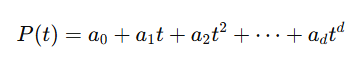
Where:

• d is the degree of the polynomial
• a₀, a₁, ..., ad are coefficients determined through least-squares fitting

This added flexibility matters because markets rarely cooperate with simple models. A degree-2 polynomial (quadratic) can capture parabolic acceleration—think of a cryptocurrency rally that starts slow and then takes off. A degree-3 polynomial (cubic) can model inflection points and S-shaped structures, where a trend reverses direction gradually. These patterns aren't exotic; they show up constantly across all markets and timeframes.

A polynomial regression channel consists of three components that work together. The center line is the fitted polynomial curve, denoted as P̂(t). This represents the estimated trend—the curved path that best fits recent price action according to the least-squares criterion. Think of it as a dynamic, curving version of a moving average.

The residuals measure the deviation of the actual price from this fitted curve:

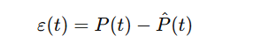
Each residual tells us how far the price strayed from the trend at a specific point. Positive residuals mean price was above the curve; negative means below. By themselves, residuals are just numbers. But when we aggregate them, they tell us something useful about volatility.

The standard deviation of these residuals provides a measure of how widely price typically fluctuates around the curved trend:

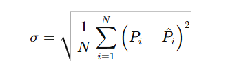
Where N is the number of observations (the lookback period).

This standard deviation is conceptually similar to what Bollinger Bands use, but with an important difference: the reference point is a curved regression line rather than a simple moving average. The bands therefore adapt not only to changes in volatility but also to changes in the shape of the trend itself.

Using this measure, the channel boundaries are defined as

Where k is a user-defined deviation multiplier. This construction creates an envelope around the curved trend line, with the width determined by recent price volatility around that curve.

Three primary parameters control how the channel behaves, and understanding them is key to using the indicator effectively.

The polynomial degree d determines how much curvature the model can express. A degree of 1 produces a straight line—identical to linear regression. This is useful as a baseline or when you specifically want a linear channel. Degree 2 allows one bend, enough to capture accelerating or decelerating trends. Degree 3 allows an S-shape, with both acceleration and deceleration within the window. Higher degrees add even more flexibility, but they come with a cost: the risk of overfitting, particularly in noisy market conditions. A polynomial that's too flexible will start fitting the noise rather than the signal, producing erratic curves that don't represent the true trend.

The lookback period N defines how many bars go into each regression calculation. This is a classic trade-off in technical analysis. Larger values smooth out noise and produce a more stable channel that changes slowly. Smaller values make the channel more responsive to recent price action, but also more sensitive to random fluctuations. There's no universal "best" setting—it depends on the instrument you're trading, the timeframe you're watching, and your personal trading style.

The deviation multiplier k controls the width of the channel. Larger values produce wider bands that contain prices more consistently. This means fewer touches of the bands and fewer signals, but the signals that do occur tend to be more significant. Smaller values produce tighter bands that price touches more frequently, which can be useful for mean-reversion strategies but also generates more false signals. In practice, traders often adjust this parameter based on the volatility of the instrument and their risk tolerance.

Once applied to a chart, the polynomial regression channel provides several layers of information. The slope of the center line indicates the direction of the trend—upward slope for uptrends, downward for downtrends. The curvature of this line reveals whether the trend is accelerating (becoming steeper) or decelerating (flattening out). The upper band acts as dynamic resistance, the lower band as dynamic support. Changes in bandwidth reflect changing volatility conditions: expanding bands indicate increasing volatility, while contracting bands suggest consolidation or decreasing volatility. A close outside the bands may signal a breakout, particularly if it follows a period of narrow, contracting bands.

By integrating these observations—slope, curvature, band width, and band touches—a trader can make more informed decisions about entries, exits, and stop placement. The channel doesn't give mechanical buy and sell signals, but it provides rich context for interpreting price action within a curved trend framework.

With the mathematical foundation laid out, the next step is translating this model into working MQL5 code. We'll use the ALGLIB numerical library to handle the heavy lifting, allowing us to focus on the indicator structure and logic rather than implementing polynomial regression from scratch.

Code Implementation

We're going to build this indicator systematically, piece by piece. Each block of code comes with an explanation of what it does and why it's structured that way. The goal isn't just to present working code—it's to help you understand the indicator deeply enough to modify it, extend it, or debug it when something doesn't work as expected.

The first part of any MQL5 indicator defines its visual appearance and chart behavior. Here we declare three plots: the center line, the upper band, and the lower band. Each gets its own color and line style—blue for the center, red for the upper, and lime green for the lower. The buffers that hold the actual line values are declared as global arrays. This is standard MQL5 practice and tells the terminal how many buffers to allocate and how to display them.

//+------------------------------------------------------------------+
//|                                  PolynomialRegressionChannel.mq5 |
//|                                Copyright 2026, Clemence Benjamin |
//|                                             https://www.mql5.com |
//+------------------------------------------------------------------+
#property copyright "Copyright 2026, Clemence Benjamin"
#property link      "https://www.mql5.com"
#property version   "1.00"
#property indicator_chart_window
#property indicator_buffers 3
#property indicator_plots   3

//--- plot Middle
#property indicator_label1  "Middle"
#property indicator_type1   DRAW_LINE
#property indicator_color1  clrBlue
#property indicator_style1  STYLE_SOLID
#property indicator_width1  1

//--- plot Upper
#property indicator_label2  "Upper"
#property indicator_type2   DRAW_LINE
#property indicator_color2  clrRed
#property indicator_style2  STYLE_SOLID
#property indicator_width2  1

//--- plot Lower
#property indicator_label3  "Lower"
#property indicator_type3   DRAW_LINE
#property indicator_color3  clrLime
#property indicator_style3  STYLE_SOLID
#property indicator_width3  1

//--- include the ALGLIB library
#include <Math\Alglib\alglib.mqh>

//--- input parameters
input int      InpDegree     = 2;           // Polynomial degree
input int      InpPeriod     = 20;          // Period (number of bars)
input double   InpDeviation  = 2.0;         // Channel deviation multiplier
input ENUM_APPLIED_PRICE InpPrice = PRICE_CLOSE; // Applied price

//--- indicator buffers
double         MiddleBuffer[];
double         UpperBuffer[];
double         LowerBuffer[];

The inclusion of the ALGLIB library deserves special attention. By adding #include <Math\Alglib\alglib.mqh>, we gain access to a professional-grade numerical library that's been rigorously tested and optimized over many years. This isn't some toy code—ALGLIB is used in scientific computing and quantitative finance worldwide. The CAlglib class provides static methods for polynomial fitting, interpolation, linear algebra, optimization, and much more. For this indicator, we'll use two functions: PolynomialFit to perform the least-squares regression, and BarycentricCalc to evaluate the fitted polynomial at any point. Both are implemented in numerically stable ways, which is essential when working with higher-degree polynomials or large datasets. Without ALGLIB, we'd have to implement our own matrix inversions and solving routines—a recipe for subtle bugs and numerical instability.

The input parameters are declared with sensible defaults that work well for initial testing. The polynomial degree defaults to 2, which is a good starting point for most markets. It allows one bend—enough to capture parabolic moves—without the overfitting risks that come with higher degrees. The period defaults to 20, a common lookback length used in many indicators. The deviation multiplier defaults to 2.0, matching the typical setting for Bollinger Bands. The price type defaults to close, but users can select any of the standard price constants through the indicator's properties window. These inputs are exposed in the UI, allowing traders to adapt the indicator to different market conditions without recompiling.

The three indicator buffers are declared as double arrays. Later we'll link them to the plots using SetIndexBuffer . These buffers are where we store the computed values for each bar; the terminal reads from these buffers to draw the lines on the chart. Keeping them as global arrays ensures they persist across function calls and are accessible throughout the indicator's lifecycle.

Now we move to the initialization function, OnInit . This function is called exactly once when the indicator is loaded onto a chart. It's the ideal place to validate input parameters, set up buffers, and perform any one-time configuration that doesn't need to be repeated on every tick.

//+------------------------------------------------------------------+
//| Custom indicator initialization function                         |
//+------------------------------------------------------------------+
int OnInit()
  {
//--- check parameters
   if(InpDegree < 1)
     {
      Print("Degree must be at least 1");
      return(INIT_PARAMETERS_INCORRECT);
     }
   if(InpPeriod < InpDegree+1)
     {
      Print("Period must be larger than degree");
      return(INIT_PARAMETERS_INCORRECT);
     }
   if(InpDeviation < 0)
     {
      Print("Deviation multiplier cannot be negative");
      return(INIT_PARAMETERS_INCORRECT);
     }

//--- set indicator buffers
   SetIndexBuffer(0, MiddleBuffer, INDICATOR_DATA);
   SetIndexBuffer(1, UpperBuffer,  INDICATOR_DATA);
   SetIndexBuffer(2, LowerBuffer,  INDICATOR_DATA);

//--- set accuracy
   IndicatorSetInteger(INDICATOR_DIGITS, _Digits);

//--- set plot labels
   PlotIndexSetString(0, PLOT_LABEL, "Middle ("+IntegerToString(InpDegree)+")");
   PlotIndexSetString(1, PLOT_LABEL, "Upper");
   PlotIndexSetString(2, PLOT_LABEL, "Lower");

//--- done
   return(INIT_SUCCEEDED);
  }

Parameter validation might seem like boilerplate, but it's actually crucial for a robust indicator. A polynomial degree less than one is mathematically meaningless—we need at least a linear fit. The period must be at least degree+1; otherwise, we have fewer data points than parameters, making the fit underdetermined and the resulting polynomial non-unique. The deviation multiplier cannot be negative because a negative width would invert the channel, putting the upper band below the lower band. If any of these conditions fail, we print a specific error message and return INIT_PARAMETERS_INCORRECT . This prevents the indicator from running with invalid settings and gives the user clear feedback about what needs fixing.

After validation, we bind the buffers to the plots using SetIndexBuffer . The second parameter, INDICATOR_DATA , tells the terminal that these are normal indicator buffers (as opposed to color buffers or other special types). We then set the number of digits displayed to match the chart's digit setting ( _Digits )—a small touch that ensures values show up with appropriate precision. Finally, we assign custom labels to each plot. The center line's label includes the chosen polynomial degree, making it easy to identify which version of the indicator is being used, especially if you have multiple instances running with different settings.

The deinitialization function, OnDeinit , is empty because we haven't allocated any dynamic resources that need manual cleanup. It's included for completeness but doesn't actually do anything.

//+------------------------------------------------------------------+
//| Custom indicator deinitialization function                       |
//+------------------------------------------------------------------+
void OnDeinit(const int reason)
  {
  }

Now we come to the heart of the indicator: the OnCalculate function. This is called on every new tick and is responsible for filling the indicator buffers with the correct values for each bar. We'll examine it in detail because this is where all the real work happens.

//+------------------------------------------------------------------+
//| Custom indicator iteration function                              |
//+------------------------------------------------------------------+
int OnCalculate(const int rates_total,
                const int prev_calculated,
                const datetime &time[],
                const double &open[],
                const double &high[],
                const double &low[],
                const double &close[],
                const long &tick_volume[],
                const long &volume[],
                const int &spread[])
  {
//--- check for minimum bars
   if(rates_total < InpPeriod)
      return(0);

//--- working arrays for ALGLIB
   double x[];
   double y[];
   ArrayResize(x, InpPeriod);
   ArrayResize(y, InpPeriod);

//--- determine start bar
   int start = prev_calculated > 0 ? prev_calculated - 1 : 0;
   if(start < InpPeriod-1)
      start = InpPeriod-1;

The first check ensures we have enough bars on the chart to form a full window. If not, we return 0, and nothing gets drawn. This is a safety measure that prevents errors when the indicator is first loaded onto a chart with insufficient historical data.

We then allocate two local arrays, x and y, each sized to the lookback period InpPeriod. These will hold the independent variable (the bar index within the current window) and the corresponding price values. Using local arrays keeps the function self-contained and avoids polluting the global namespace with temporary variables.

The determination of the starting bar is a performance optimization that's worth understanding. The prev_calculated parameter tells us how many bars were already processed in the previous call to OnCalculate. If it's greater than zero, we only need to update the most recent bar—the one at index prev_calculated - 1. Otherwise, we're starting from scratch and need to process all bars where a full window is available, which is from index InpPeriod - 1 onward. This logic ensures we don't waste CPU time recalculating the entire history on every tick, which would be especially wasteful on high-frequency charts.

//--- main loop
   for(int i = start; i < rates_total; i++)
     {
      //--- fill x and y arrays (x = 0 .. period-1, y = price values)
      for(int j = 0; j < InpPeriod; j++)
        {
         x[j] = j;  // use integer indices as regressor
         y[j] = GetPrice(InpPrice, open, high, low, close, i - InpPeriod + 1 + j);
        }

Inside the main loop, for each bar index i, we have to fill the x and y arrays with the data for the regression window ending at that bar. The independent variable x is simply the index j from 0 to InpPeriod-1. You might wonder why we use simple indices rather than actual timestamps or bar numbers. The answer is that polynomial regression is invariant under translation and scaling of the independent variable—shifting all x-values by a constant or multiplying them by a scalar doesn't change the shape of the fitted curve, only the coefficient values. Using 0, 1, 2,… keeps the numbers small and avoids numerical issues that could arise with large UNIX timestamps. It also means the polynomial coefficients are independent of the actual bar times, which is a desirable property for a chart indicator.

The corresponding y values are obtained by calling the helper function GetPrice with the appropriate price arrays and the index i - InpPeriod + 1 + j. This expression might look complicated, but it's just calculating the bar index within the chart's history that corresponds to position j in the current window. As j runs from 0 to InpPeriod-1, this index runs from i - InpPeriod + 1 to i—exactly the last InpPeriod bars ending at the current bar i. Each bar gets its own unique window, which slides forward as we move through the loop.

      //--- create ALGLIB objects for polynomial fit
      CBarycentricInterpolantShell p;
      CPolynomialFitReportShell rep;
      int info;

      //--- call polynomial fitting (degree = InpDegree => m = InpDegree+1)
      CAlglib::PolynomialFit(x, y, InpPeriod, InpDegree+1, info, p, rep);

Now we prepare to call ALGLIB. We instantiate three objects: p of type CBarycentricInterpolantShell, which will hold the fitted polynomial in a form that can be efficiently evaluated; rep of type CPolynomialFitReportShell , which can contain additional information about the fit (though we don't use it here); and an integer info that will receive a status code from the fitting routine.

The call to CAlglib::PolynomialFit takes the x and y arrays, the number of points (InpPeriod), the number of basis functions (which is InpDegree+1 for a polynomial of degree InpDegree), and references to info , p , and rep. The function performs a least-squares fit of a polynomial of the specified degree to the data and returns a status code in info. A positive value indicates success; zero or negative values indicate various error conditions—insufficient data, singular matrix, numerical issues, and so on.

      //--- if fitting succeeded, compute channel
      if(info > 0)
        {
         //--- compute fitted values for all points in the window
         double fitted[];
         ArrayResize(fitted, InpPeriod);
         double sum_sq = 0.0;

         for(int j = 0; j < InpPeriod; j++)
           {
            fitted[j] = CAlglib::BarycentricCalc(p, x[j]);
            double resid = y[j] - fitted[j];
            sum_sq += resid * resid;
           }

If the fit succeeded (indicated by info > 0 ), we allocate a temporary array fitted to hold the fitted values for each point in the window. We then loop over all points in the window, calling CAlglib::BarycentricCalc(p, x[j]) to evaluate the fitted polynomial at each x[j]. This gives us the fitted price at that point. The residual is the difference between the actual price ( y[j] ) and the fitted value. We square each residual and accumulate the sum of squares in sum_sq.

You might wonder why we need fitted values for all points in the window rather than just the current point. The reason is that we need the standard deviation of the residuals across the entire window to calculate the channel width. The standard deviation is a measure of the typical deviation of price from the fitted curve, and computing it over all points in the window gives us a robust estimate of the current volatility around the trend.

         //--- standard deviation of residuals
         double stddev = MathSqrt(sum_sq / (InpPeriod - InpDegree - 1));  // unbiased

The standard deviation calculation deserves careful attention. We compute it as the square root of the variance, where the variance is sum_sq / (n - d - 1). Here n is the period and d is the degree. This is the unbiased estimator, which uses n - d - 1 degrees of freedom because we have estimated d+1 parameters (the polynomial coefficients) from the data. The denominator is smaller than n , which increases the estimated variance slightly—this adjustment is important when the sample size is small because it gives a more accurate estimate of the true population variance. Without this correction, the channel would be slightly too narrow, especially for shorter lookback periods.

         //--- value at the current point (x = InpPeriod-1)
         double middle = CAlglib::BarycentricCalc(p, InpPeriod-1);
         MiddleBuffer[i] = middle;
         UpperBuffer[i]  = middle + InpDeviation * stddev;
         LowerBuffer[i]  = middle - InpDeviation * stddev;
        }

The center line value at the current bar is simply the polynomial evaluated at the last point in the window, where x = InpPeriod-1. We store this value in MiddleBuffer[i]. The upper and lower bands are then calculated as middle ± InpDeviation * stddev. These values go into their respective buffers, and the terminal will use them to draw the lines on the chart.

      else
        {
         //--- fitting failed, copy previous values or set empty
         if(i > 0)
           {
            MiddleBuffer[i] = MiddleBuffer[i-1];
            UpperBuffer[i]  = UpperBuffer[i-1];
            LowerBuffer[i]  = LowerBuffer[i-1];
           }
         else
           {
            MiddleBuffer[i] = 0.0;
            UpperBuffer[i]  = 0.0;
            LowerBuffer[i]  = 0.0;
           }
        }
     }

//--- return value of prev_calculated for next call
   return(rates_total);
  }

If the fit failed—which is rare but possible with degenerate data, such as constant prices over the entire window—we need to handle it gracefully. For bars after the first, we simply copy the previous bar's values forward. This ensures the channel remains continuous and doesn't produce distracting gaps. For the very first bar (which can only happen if the window is full but the fit still fails), we set the values to zero. In practice, such failures are so uncommon that this simple fallback is perfectly adequate.

Finally, we return rates_total. This becomes the new prev_calculated value on the next call to OnCalculate , enabling the optimization logic we set up earlier to work correctly—only the most recent bar will need recalculation on subsequent ticks.

The helper function GetPrice is straightforward but worth including to keep the main loop clean. It takes a price type enumeration and the price arrays and returns the appropriate value for the given index. This makes it easy to add more price types in the future without cluttering the main calculation logic.

//+------------------------------------------------------------------+
//| Helper function to get price based on ENUM_APPLIED_PRICE         |
//+------------------------------------------------------------------+
double GetPrice(ENUM_APPLIED_PRICE price_type,
                const double &open[],
                const double &high[],
                const double &low[],
                const double &close[],
                int index)
  {
   switch(price_type)
     {
      case PRICE_CLOSE:   return close[index];
      case PRICE_OPEN:    return open[index];
      case PRICE_HIGH:    return high[index];
      case PRICE_LOW:     return low[index];
      case PRICE_MEDIAN:  return (high[index] + low[index]) / 2.0;
      case PRICE_TYPICAL: return (high[index] + low[index] + close[index]) / 3.0;
      case PRICE_WEIGHTED:return (high[index] + low[index] + 2*close[index]) / 4.0;
      default:              return close[index];
     }
  }
//+------------------------------------------------------------------+

The code is now complete. It's efficient, robust, and clearly structured. Every component has been explained, from the high-level concept down to the low-level implementation details. With this foundation, you can compile the indicator and start testing it on real charts.

Testing

Once compiled (F7 in MetaEditor), drag the indicator onto any chart. You'll see three lines: blue center, red upper band, and green lower band.

Start with EURUSD H1, default settings (degree 2, period 20, deviation 2.0, close). Scroll back and watch how the center line curves—it bends to follow price, unlike a straight linear regression channel.

Testing the Polynomial Regression Channel in Strategy Tester

Now experiment with parameters. Drop period to 10—more responsive but noisier. Bump to 50—smoother but slower. Switch the degree to 1 for linear regression baseline, then to 2 or 3 on a parabolic move to see the curve follow acceleration better (but watch for overfitting with degree 3).

Adjust deviation multiplier: 1.5 tightens bands for mean-reversion signals; 2.5 widens them, making breakouts more significant. Try different price types—high shifts channel up (resistance), low shifts down (support).

Test on different instruments. Bands widen automatically during volatile news events, tighten in quiet periods—built into the math.

Interpretation takes practice. Price at upper band: strong enough to break or reversing? Look for candlestick confirmation. Slope and curvature of the center line add context—steepening suggests momentum, and flattening warns of exhaustion.

Use it like any channel: visual analysis, stop placement, or part of a larger system. Experiment to learn its strengths.

Conclusion

We started from a practical problem—linear channels fail to represent curved market structure—and delivered a concrete, testable solution: a polynomial regression channel implemented in MQL5 that you can compile and attach to any chart. Using ALGLIB allowed us to rely on robust numerical routines (polynomial fitting and barycentric evaluation) instead of reimplementing fragile linear-algebra code. The indicator includes input validation (degree ≥ 1, period > degree, non-negative deviation), an unbiased standard-deviation estimator that accounts for estimated parameters, and graceful fallbacks when a fit fails.

On the operational side, the implementation minimizes runtime overhead by recalculating only the newest bar when possible, uses small, translated x-values (0.. N-1) to avoid numerical scaling issues, and stores results in standard indicator buffers for immediate charting or programmatic consumption. Default parameter guidance (degree = 2, period ≈ 20, deviation ≈ 2.0) provides a sensible starting point, while explicit warnings about overfitting clarify when higher degrees are inappropriate for noisy data.

What you receive is a production-ready artifact (PolynomialRegressionChannel.mq5) and a clear pattern for extension: add band-touch alerts, color bands by slope or curvature, expose curvature metrics for signal rules, or use the center and bands as building blocks inside an EA. Use the channel for visual context, stop placement, or as a reproducible filter in automated strategies—always mindful of parameter trade-offs (responsiveness vs. stability) and the risk of fitting noise when increasing polynomial degree.

Attachments

File Name	Type	Version	Description
PolynomialRegressionChannel.mq5	Indicator	1.00	Complete MQL5 source code for the polynomial regression channel indicator. It uses the ALGLIB library to perform polynomial least-squares fitting and draws an adaptive trend channel with center, upper, and lower lines. The code includes full input validation, efficient sliding-window calculation that recalculates only when necessary, and a helper function for selecting different price types. The unbiased standard deviation estimator ensures accurate channel widths even with shorter lookback periods.