Fast trading strategy tester in Python using Numba

Why a fast custom strategy tester is important

When developing trading algorithms based on machine learning, it is important to correctly and quickly evaluate the results of their trading on history. If we take into account the rare use of the tester on large time intervals and with a small history depth, then the tester in Python is quite suitable. However, if the task involves multiple tests and high-frequency strategies, then an interpreted language may be too slow.

Let's say we are not satisfied with the execution speed of some scripts, but we do not want to give up our familiar Python development environment. This is where Numba comes to the rescue, allowing us to convert and compile native Python code into fast machine code on the fly. The execution speed of such a code becomes comparable to the execution speed of code in programming languages, such as C and FORTRAN.

Brief description of the Numba library

Numba is a library for the Python programming language designed to speed up code execution by compiling functions at the bytecode level into machine code using JIT (Just-In-Time) compilation. This technology can significantly improve computing performance, especially in scientific applications that frequently use loops and complex mathematical operations. The library supports working with NumPy arrays and also allows for efficient work with parallelism and GPU computing. 

The most common way to use Numba is to apply its collection of decorators to Python functions to tell Numba to compile them. When a function decorated with Numba is called, it is compiled to machine code just in time, allowing all or part of the code to run at the speed of native machine code.

The following architectures are currently supported:

• OS: Windows (64 bit), OSX, Linux (64 bit).

• Architecture: x86, x86_64, ppc64le, armv8l (aarch64), M1/Arm64.

• GPUs: Nvidia CUDA.

• CPython

• NumPy 1.22 - 1.26

It is worth considering that the Pandas package is not supported by the Numba library, and working with dataframes will be performed at the same speed. 

Handling article codes

To make everything work right away, take the following preliminary steps:

• install all necessary packages;
  

pip install numpy
pyp install pandas
pip install catboost
pip install scikit-learn
pip install scipy

• download EURGBP_H1.csv data and place it in the Files folder;
• download all Python scripts and put them in one folder;
• edit the first string of Tester_ML.py, so that it looks like this: from tester_lib import test_model;
• specify the path to the file in the Tester_ML.py script;
• p = pd.read_csv('C:/Program Files/MetaTrader 5/MQL5/Files/'EURGBP_H1'.csv', sep='\s+').

How to use Numba package?

In general, using the Numba package boils down to installing it

pip install numba
conda install numba

and applying the decorator before the function we want to speed up, for example:

@jit(nopython=True)
def process_data(*args):
        ...

The decorator is called in two different ways. 

1. nopython mode
2. object mode

The first way is to compile the decorated function so that it runs entirely without involving the Python interpreter. This is the fastest method and is recommended for use. However, Numba has limitations, such as being able to compile only Python's built-in operations and Numpy array operations. If a function contains objects from other libraries, such as Pandas, Numba will not be able to compile it and the code will be executed by the interpreter.

Numba can use object mode to get around restrictions on using third-party libraries. In this mode, Numba will compile the function, assuming everything is a Python object, and essentially run the code in the interpreter.

@jit(forceobj=true, looplift=True)

may improve performance compared to pure object mode, since Numba will attempt to compile loops into functions that execute in machine code and run the rest of the code in the interpreter. For best performance, avoid using object mode altogether!

The package also supports parallel computing when possible (Parallel=True). Please note that the first time a function is called, it is compiled into machine code, which takes some time. This code will then be cached and subsequent calls will be faster.

Example of speeding up the deal markup function

Before we start speeding up the tester, let's try speeding up something simpler. A great candidate for this role is the deal markup function. This function takes a dataframe with prices and marks the trades as buy and sell (0 and 1). Such functions are often used to pre-label data, so that a classifier can be trained later.

def get_labels(dataset, min = 1, max = 15) -> pd.DataFrame:
    labels = []
    for i in range(dataset.shape[0]-max):
        rand = random.randint(min, max)
        curr_pr = dataset['close'].iloc[i]
        future_pr = dataset['close'].iloc[i + rand]

        if (future_pr + hyper_params['markup']) < curr_pr:
            labels.append(1.0)
        elif (future_pr - hyper_params['markup']) > curr_pr:
            labels.append(0.0)
        else:
            labels.append(2.0)
        
    dataset = dataset.iloc[:len(labels)].copy()
    dataset['labels'] = labels
    dataset = dataset.dropna()
    dataset = dataset.drop(
        dataset[dataset.labels == 2.0].index)
    return dataset

We use minute closing prices of the EURGBP for 15 years as data:

>>> pr = get_prices()
>>> pr
                       close
time                        
2010-01-04 00:00:00  0.88810
2010-01-04 00:01:00  0.88799
2010-01-04 00:02:00  0.88786
2010-01-04 00:03:00  0.88792
2010-01-04 00:04:00  0.88802
...                      ...
2024-10-09 19:03:00  0.83723
2024-10-09 19:04:00  0.83720
2024-10-09 19:05:00  0.83704
2024-10-09 19:06:00  0.83702
2024-10-09 19:07:00  0.83703

[5480021 rows x 1 columns]

The dataset contains more than five million observations, which is quite sufficient for testing.

Now let's measure the execution speed of this function on our data:

# get labels test
start_time = time.time()
pr = get_labels(pr)
pr['meta_labels'] = 1.0
end_time = time.time()
execution_time = end_time - start_time
print(f"Execution time: {execution_time:.4f} seconds")

The execution time was 74.1843 seconds.

Now let's try to speed up this function using the Numba package. We can see that the original function also uses the Pandas package, and we know that these two packages are incompatible. Let's move everything related to Pandas into a separate function and speed up the rest of the code.

@jit(nopython=True)
def get_labels_numba(close_prices, min_val, max_val, markup):
    labels = np.empty(len(close_prices) - max_val, dtype=np.float64)
    for i in range(len(close_prices) - max_val):
        rand = np.random.randint(min_val, max_val + 1)
        curr_pr = close_prices[i]
        future_pr = close_prices[i + rand]

        if (future_pr + markup) < curr_pr:
            labels[i] = 1.0
        elif (future_pr - markup) > curr_pr:
            labels[i] = 0.0
        else:
            labels[i] = 2.0

    return labels

def get_labels_fast(dataset, min_val=1, max_val=15):
    close_prices = dataset['close'].values
    markup = hyper_params['markup']

    labels = get_labels_numba(close_prices, min_val, max_val, markup)

    dataset = dataset.iloc[:len(labels)].copy()
    dataset['labels'] = labels
    dataset = dataset.dropna()
    dataset = dataset.drop(dataset[dataset.labels == 2.0].index)

    return dataset

The first function is preceded by a call to the @jit decorator. This means that this function will be compiled into byte code. We also get rid of Pandas inside it and use only lists, loops and Numpy.

The second function does the preparatory work. It converts the Pandas dataframe into a Numpy array and then passes it to the first function. After that, it takes the result and returns the Pandas dataframe again. This way, the markup main calculation will be accelerated.

Now let's measure the speed. Calculation time has been reduced to 12 seconds! For this function, we got more than 5x speedup. Of course, this is not a completely clean test, since the Pandas library is still used for intermediate calculations, but significant speedup was achieved in terms of label calculation.

Speeding up the strategy tester for machine learning tasks

I moved the strategy tester to a separate library, which can be found in the attachment below. It contains 'tester' and 'slow_tester' functions for comparison.

The reader might object that most of the speedups in Python come from vectorization. This is true, but sometimes we still have to use loops. For example, the tester has a fairly complex loop for going through the entire history and accumulating the total profit, taking into account stop loss and take profit. Implementing this through vectorization does not seem like a simple task.

The body of the tester loop (the part that takes the longest to execute) is shown below for reference purposes.

for i in range(dataset.shape[0]):
        line_f = len(report) if i <= forw else line_f
        line_b = len(report) if i <= backw else line_b
        
        pred = labels[i]
        pr = close[i]
        pred_meta = metalabels[i]  # 1 = allow trades

        if last_deal == 2 and pred_meta == 1:
            last_price = pr
            last_deal = 0 if pred < 0.5 else 1
            continue
        
        if last_deal == 0:
            if (-markup + (pr - last_price) >= take) or (-markup + (last_price - pr) >= stop):
                last_deal = 2
                profit = -markup + (pr - last_price)
                report.append(report[-1] + profit)
                chart.append(chart[-1] + profit)
                continue

        if last_deal == 1:
            if (-markup + (pr - last_price) >= stop) or (-markup + (last_price - pr) >= take):
                last_deal = 2
                profit = -markup + (last_price - pr)
                report.append(report[-1] + profit)
                chart.append(chart[-1] + (pr - last_price))
                continue
        
        # close deals by signals
        if last_deal == 0 and pred > 0.5 and pred_meta == 1:
            last_deal = 2
            profit = -markup + (pr - last_price)
            report.append(report[-1] + profit)
            chart.append(chart[-1] + profit)
            continue

        if last_deal == 1 and pred < 0.5 and pred_meta == 1:
            last_deal = 2
            profit = -markup + (last_price - pr)
            report.append(report[-1] + profit)
            chart.append(chart[-1] + (pr - last_price))
            continue

Let's measure the test speed on the data we received before. First, let's look at the speed of the slow tester:

# native python tester test
start_time = time.time()
tester_slow(pr, 
       hyper_params['stop_loss'], 
       hyper_params['take_profit'], 
       hyper_params['markup'],
       hyper_params['forward'],
       False)
end_time = time.time()
execution_time = end_time - start_time
print(f"Execution time: {execution_time:.4f} seconds")

Execution time: 6.8639 seconds

It does not look very slow, one could even say that the interpreter executes the code quite quickly.

Let's split the tester function into two functions again. One will be auxiliary, and the second will perform the main calculations.

The 'process data' function implements the main loop of the tester, which should be accelerated, since loops in Python are slow. At the same time, the 'tester' function itself first prepares data for the 'process data' function, then accepts the result and draws the graph.

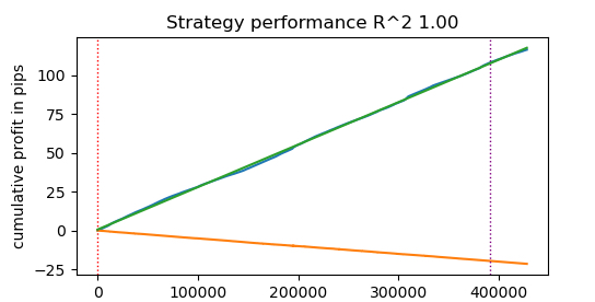
@jit(nopython=True)
def process_data(close, labels, metalabels, stop, take, markup, forward, backward):
    last_deal = 2
    last_price = 0.0
    report = [0.0]
    chart = [0.0]
    line_f = 0
    line_b = 0

    for i in range(len(close)):
        line_f = len(report) if i <= forward else line_f
        line_b = len(report) if i <= backward else line_b
        
        pred = labels[i]
        pr = close[i]
        pred_meta = metalabels[i]  # 1 = allow trades

        if last_deal == 2 and pred_meta == 1:
            last_price = pr
            last_deal = 0 if pred < 0.5 else 1
            continue
        
        if last_deal == 0:
            if (-markup + (pr - last_price) >= take) or (-markup + (last_price - pr) >= stop):
                last_deal = 2
                profit = -markup + (pr - last_price)
                report.append(report[-1] + profit)
                chart.append(chart[-1] + profit)
                continue

        if last_deal == 1:
            if (-markup + (pr - last_price) >= stop) or (-markup + (last_price - pr) >= take):
                last_deal = 2
                profit = -markup + (last_price - pr)
                report.append(report[-1] + profit)
                chart.append(chart[-1] + (pr - last_price))
                continue
        
        # close deals by signals
        if last_deal == 0 and pred > 0.5 and pred_meta == 1:
            last_deal = 2
            profit = -markup + (pr - last_price)
            report.append(report[-1] + profit)
            chart.append(chart[-1] + profit)
            continue

        if last_deal == 1 and pred < 0.5 and pred_meta == 1:
            last_deal = 2
            profit = -markup + (last_price - pr)
            report.append(report[-1] + profit)
            chart.append(chart[-1] + (pr - last_price))
            continue

    return np.array(report), np.array(chart), line_f, line_b

def tester(*args):
    '''
    This is a fast strategy tester based on numba
    List of parameters:

    dataset: must contain first column as 'close' and last columns with "labels" and "meta_labels"

    stop: stop loss value

    take: take profit value

    forward: forward time interval

    backward: backward time interval

    markup: markup value

    plot: false/true
    '''
    dataset, stop, take, forward, backward, markup, plot = args

    forw = dataset.index.get_indexer([forward], method='nearest')[0]
    backw = dataset.index.get_indexer([backward], method='nearest')[0]

    close = dataset['close'].to_numpy()
    labels = dataset['labels'].to_numpy()
    metalabels = dataset['meta_labels'].to_numpy()
    
    report, chart, line_f, line_b = process_data(close, labels, metalabels, stop, take, markup, forw, backw)

    y = report.reshape(-1, 1)
    X = np.arange(len(report)).reshape(-1, 1)
    lr = LinearRegression()
    lr.fit(X, y)

    l = 1 if lr.coef_[0][0] >= 0 else -1

    if plot:
        plt.plot(report)
        plt.plot(chart)
        plt.axvline(x=line_f, color='purple', ls=':', lw=1, label='OOS')
        plt.axvline(x=line_b, color='red', ls=':', lw=1, label='OOS2')
        plt.plot(lr.predict(X))
        plt.title("Strategy performance R^2 " + str(format(lr.score(X, y) * l, ".2f")))
        plt.xlabel("the number of trades")
        plt.ylabel("cumulative profit in pips")
        plt.show()

    return lr.score(X, y) * l

Now let's test the Numba-accelerated strategy tester:

start_time = time.time()
tester(pr, 
       hyper_params['stop_loss'], 
       hyper_params['take_profit'], 
       hyper_params['forward'],
       hyper_params['backward'],
       hyper_params['markup'],
       False)
end_time = time.time()
execution_time = end_time - start_time
print(f"Execution time: {execution_time:.4f} seconds")

Execution time: 0.1470 seconds

The observed speed increase is almost 50 times! More than 400,000 deals were completed.

Imagine that if you spent 1 hour a day testing your algorithms, then with the fast tester it would take you only one minute.

Testing strategies on tick data

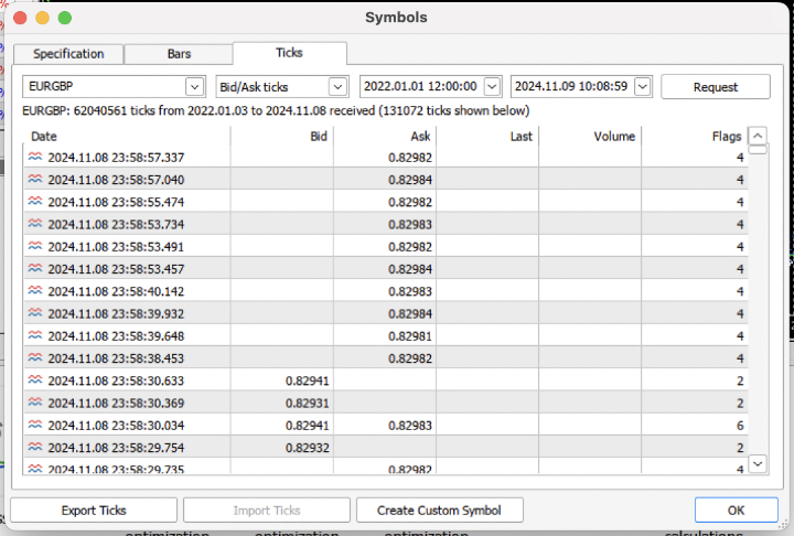
Let's complicate the task and download the tick history for the last 3 years from the terminal into a .csv file.

To read the file correctly, the quote loading function should be slightly modified. Instead of Close, we will use Bid prices. We also need to remove prices with the same indices.

def get_prices() -> pd.DataFrame:
    p = pd.read_csv('files/'+hyper_params['symbol']+'.csv', sep='\s+')
    pFixed = pd.DataFrame(columns=['time', 'close'])
    pFixed['time'] = p['<DATE>'] + ' ' + p['<TIME>']
    pFixed['time'] = pd.to_datetime(pFixed['time'], format='mixed')
    pFixed['close'] = p['<BID>']
    pFixed.set_index('time', inplace=True)
    pFixed.index = pd.to_datetime(pFixed.index, unit='s')
    # Remove duplicate string by 'time' index
    pFixed = pFixed[~pFixed.index.duplicated(keep='first')]
    return pFixed.dropna()

The result was almost 62 million observations. The tester accepts prices by the column name "close", so Bid is renamed to Close.

>>> pr
                           close
time                            
2022-01-03 00:05:01.753  0.84000
2022-01-03 00:05:04.032  0.83892
2022-01-03 00:05:05.849  0.83918
2022-01-03 00:05:07.280  0.83977
2022-01-03 00:05:07.984  0.83939
...                          ...
2024-11-08 23:58:53.491  0.82982
2024-11-08 23:58:53.734  0.82983
2024-11-08 23:58:55.474  0.82982
2024-11-08 23:58:57.040  0.82984
2024-11-08 23:58:57.337  0.82982

[61896607 rows x 1 columns]

Let's run a quick markup and measure the execution time.

# get labels test
start_time = time.time()
pr = get_labels_fast(pr)
pr['meta_labels'] = 1.0
end_time = time.time()
execution_time = end_time - start_time
print(f"Execution time: {execution_time:.4f} seconds")

The markup time was 9.5 seconds.

Now let's run the fast tester.

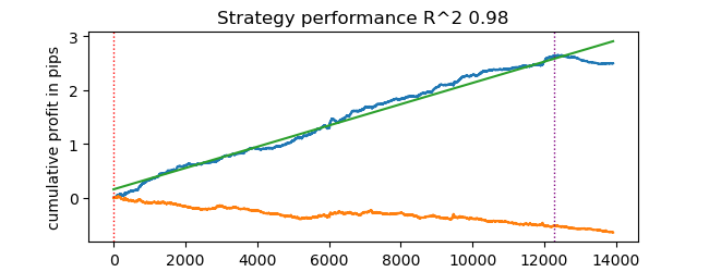
# numba tester test
start_time = time.time()
tester(pr, 
       hyper_params['stop_loss'], 
       hyper_params['take_profit'], 
       hyper_params['forward'],
       hyper_params['backward'],
       hyper_params['markup'],
       True)
end_time = time.time()
execution_time = end_time - start_time
print(f"Execution time: {execution_time:.4f} seconds")

The test time took 0.16 seconds. While the slow tester spent 5.5 seconds on this.

The fast tester on Numba completed the task 35 times faster than the tester on pure Python. In fact, from the observer's point of view, testing happens instantly in the case of the fast tester, whereas using the slow one requires some waiting. Still, it is worth giving credit to the slow tester, which also does a good job and is quite suitable for testing strategies even on tick data.

In total, there were 1e6 or one million deals.

 

Information on using the fast tester for machine learning tasks

If you are actually going to use the suggested tester, then the following information may be useful to you.

Let's add features to our dataset so that we can train the classifier.

def get_features(data: pd.DataFrame) -> pd.DataFrame:
    pFixed = data.copy()
    pFixedC = data.copy()
    count = 0
    for i in hyper_params['periods']:
        pFixed[str(count)] = pFixedC-pFixedC.rolling(i).mean()
        count += 1
    return pFixed.dropna()

These are simple indicators based on the difference in prices and moving averages.

Next, we create a dictionary of model hyperparameters that will be used for training and testing. We will apply them when generating a new dataset.

hyper_params = {
    'symbol': 'EURGBP_H1',
    'markup': 0.00010,
    'stop_loss': 0.01000,
    'take_profit': 0.01000,
    'backward': datetime(2010, 1, 1),
    'forward': datetime(2023, 1, 1),
    'periods': [i for i in range(50, 300, 50)],
}

# catboost learning
dataset = get_labels_fast(get_features(get_prices()))
dataset['meta_labels'] = 1.0
data = dataset[(dataset.index < hyper_params['forward']) & (dataset.index > hyper_params['backward'])].copy()

Here it is worth paying attention to the fact that the tester accepts not only the "labels" values, but also "meta_labels" ones. We might need them if we want to use filters for our machine learning-based trading system. Then the value of 1 will allow trading, and the value of 0 will prohibit it. Since we will not be using filters in this demo example, we will just create an extra column and fill it with ones allowing trading at all times.

dataset['meta_labels'] = 1.0

Now we can train the CatBoost model on the generated dataset, having previously removed the forward and backward test data from the history so that it does not train on them.

data = dataset[(dataset.index < hyper_params['forward']) & (dataset.index > hyper_params['backward'])].copy()

X = data[data.columns[1:-2]]
y = data['labels']

train_X, test_X, train_y, test_y = train_test_split(
        X, y, train_size=0.7, test_size=0.3, shuffle=True)

model = CatBoostClassifier(iterations=500,
                               thread_count=8,
                               custom_loss=['Accuracy'],
                               eval_metric='Accuracy',
                               verbose=True,
                               use_best_model=True,
                               task_type='CPU')

model.fit(train_X, train_y, eval_set=(test_X, test_y),
            early_stopping_rounds=25, plot=False)

After training, test the model on the entire dataset, including test data. The test_model function is located in the tester_lib.py file along with the functions of the fast and slow tester itself. It is a wrapper for the fast tester and performs the task of obtaining predicted values of a trained machine learning model (in our case it is CatBoost, but it might be any other).

def test_model(dataset: pd.DataFrame, 
               result: list, 
               stop: float, 
               take: float, 
               forward: float, 
               backward: float, 
               markup: float, 
               plt = False):
    
    ext_dataset = dataset.copy()
    X = ext_dataset[dataset.columns[1:-2]]

    ext_dataset['labels'] = result[0].predict_proba(X)[:,1]
    # ext_dataset['meta_labels'] = result[1].predict_proba(X)[:,1]
    ext_dataset['labels'] = ext_dataset['labels'].apply(lambda x: 0.0 if x < 0.5 else 1.0)
    # ext_dataset['meta_labels'] = ext_dataset['meta_labels'].apply(lambda x: 0.0 if x < 0.5 else 1.0)
    return tester(ext_dataset, stop, take, forward, backward, markup, plt)

The code above has commented out strings that allow you to get meta labels responsible for indicating whether to trade/not to trade. In other words, the second machine learning model can be used for these purposes. We do not use it in this article.

Let's start testing directly.

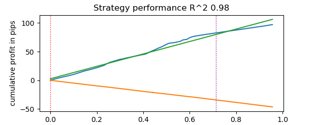
# test catboost model
test_model(dataset, 
           [model], 
           hyper_params['stop_loss'],
           hyper_params['take_profit'],
           hyper_params['forward'],
           hyper_params['backward'],
           hyper_params['markup'],
           True)

And we get the result. The model has been overfitted, as can be seen in the test data to the right of the vertical line. But that does not matter for us, because we are testing the tester.

Since the tester implies the possibility of using stop loss and take profit, and you may want to optimize them, then let's use optimization, because our tester is now very fast!

Optimization of trading system parameters using machine learning

Now let's look at the possibility of optimizing stop loss and take profit. In fact, it is possible to optimize other parameters of the trading system, such as meta labels, but this is beyond the scope of this article and can be discussed in the next one.

We implement two types of optimization:

• Search by parameter grid
• Optimization using the L-BFGS-B method

Let's first briefly go over the code for each method. The GRID_SEARCH method is displayed below. 

It takes as arguments:

• dataset for testing
• trained model
• the dictionary containing the hyperparameters of the algorithm described above
• tester object

Next, ranges of parameter values are created that will be iterated over, and they are iterated over in a loop. At each iteration, the tester is called and those parameters that correspond to the largest R^2 are selected.

# stop loss / take profit grid search
def optimize_params_GRID_SEARCH(pr, model, hyper_params, test_model_func):
    best_r2 = -np.inf
    best_stop_loss = None
    best_take_profit = None

    # Ranges for stop_loss and take_profit
    stop_loss_range = np.arange(0.00100, 0.02001, 0.00100)
    take_profit_range = np.arange(0.00100, 0.02001, 0.00100)

    total_iterations = len(stop_loss_range) * len(take_profit_range)
    start_time = time.time()

    for stop_loss in stop_loss_range:
        for take_profit in take_profit_range:
            # Create a copy of hyper_params
            current_hyper_params = hyper_params.copy()
            current_hyper_params['stop_loss'] = stop_loss
            current_hyper_params['take_profit'] = take_profit

            r2 = test_model_func(pr,
                                 [model],
                                 current_hyper_params['stop_loss'],
                                 current_hyper_params['take_profit'],
                                 current_hyper_params['forward'],
                                 current_hyper_params['backward'],
                                 current_hyper_params['markup'],
                                 False)

            if r2 > best_r2:
                best_r2 = r2
                best_stop_loss = stop_loss
                best_take_profit = take_profit

    end_time = time.time()
    total_time = end_time - start_time
    average_time_per_iteration = total_time / total_iterations

    print(f"Total iterations: {total_iterations}")
    print(f"Average time per iteration: {average_time_per_iteration:.6f} seconds")
    print(f"Total time: {total_time:.6f} seconds")

    return best_stop_loss, best_take_profit, best_r2

Now let's look at the code of the L-BFGS_B method. Find more detailed information on it here. 

The function arguments remain the same. But it creates a fitness function the strategy tester is called through. The boundaries of the optimization parameters and the number of initializations (random points of the parameter set) for the L-BFGS_B algorithm are specified. Random initializations are needed to prevent the optimization algorithm from getting stuck in local minima. After this, the minimize function is called the parameters of the optimizer itself are passed to.

def optimize_params_L_BFGS_B(pr, model, hyper_params, test_model_func):
    def objective(x):
        current_hyper_params = hyper_params.copy()
        current_hyper_params['stop_loss'] = x[0]
        current_hyper_params['take_profit'] = x[1]
        
        r2 = test_model_func(pr,
                            [model],
                            current_hyper_params['stop_loss'],
                            current_hyper_params['take_profit'],
                            current_hyper_params['forward'],
                            current_hyper_params['backward'],
                            current_hyper_params['markup'],
                            False)
        return -r2

    bounds = ((0.001, 0.02), (0.001, 0.02))
    
    # Let's try some random starting points
    n_attempts = 50
    best_result = None
    best_fun = float('inf')
    
    start_time = time.time()
    for _ in range(n_attempts):
        # Random starting point
        x0 = np.random.uniform(0.001, 0.02, 2)
        
        result = minimize(
            objective,
            x0,
            method='L-BFGS-B',
            bounds=bounds,
            options={'ftol': 1e-5, 'disp': False, 'maxiter': 100}  # Increase accuracy and number of iterations
        )
        
        if result.fun < best_fun:
            best_fun = result.fun
            best_result = result
    # Get the end time and calculate the total time
    end_time = time.time()
    total_time = end_time - start_time
    print(f"Total time: {total_time:.6f} seconds")

    return best_result.x[0], best_result.x[1], -best_result.fun

Now we can run both optimization algorithms and look at the execution time and accuracy.

# using
best_stop_loss, best_take_profit, best_r2 = optimize_params_GRID_SEARCH(dataset, model, hyper_params, test_model)
best_stop_loss, best_take_profit, best_r2 = optimize_params_L_BFGS_B(dataset, model, hyper_params, test_model)

Grid search algorithm:

Total iterations: 400
Average time per iteration: 0.031341 seconds
Total time: 12.536394 seconds

Best parameters: stop_loss=0.004, take_profit=0.002, R^2=0.9742298702323458

L-BFGS-B algorithm:

Total time: 4.733158 seconds

Best parameters: stop_loss=0.0030492548809269732, take_profit=0.0016816794762543421, R^2=0.9733045271274298

With my standard settings, L-BFGS-B performed more than 2 times faster, showing results comparable to the grid search algorithm.

Thus, one can use both of these algorithms and choose the best one depending on the number and range of parameters to be optimized. 

Conclusion

This article demonstrates the possibility of accelerating the strategy tester, which can be used to quickly test machine learning-based strategies. Numba has been shown to provide the 50x speed boost. Testing becomes fast, allowing for multiple tests and even parameter optimization. 

Attachments:

• tester_lib.py - tester library
• test tester.py - script for comparing slow (Python) and fast (Numba) testers
• tester ticks.py - script for comparing testers on tick data
• tester ML.py - script for classifier training and hyperparameter optimization