Exploring Machine Learning in Unidirectional Trend Trading Using Gold as a Case Study

Introduction

Recently, we have been studying implementation of symmetrical trading systems through the lens of binary classification. We assumed that buy and sell transactions can be well separated in the feature space, that is, there is some dividing line (hyperplane) that enables the machine learning algorithm to predict both long and short positions equally well.

In reality, this is not always the case, especially for trending trading instruments such as some metals and indices, as well as cryptocurrencies. In situations where an asset has a clearly defined unidirectional trend, trading systems that imply buys and sells may be too risky. And the overall distribution of such trades may be highly asymmetric, leading to misclassification with a large number of errors.

In this case, a bidirectional trading system may be ineffective, and it would be better to focus on trading in one direction. This article aims to shed light on features of machine learning to create such unidirectional strategies.

I suggest that approaches of causal inference must be reimagined and adapted to the task of unidirectional trading.

Let's take materials from previous articles as a basis:

• Cross-validation and basics of causal inference in CatBoost models, export to ONNX format
• Causal inference in time series classification problems
• Fast trading strategy tester in Python using Numba

I strongly recommend reading these articles for a more complete understanding of the idea of causal inference and testing.

Creating a sampler of trades in a given direction

Since we used to mark up buy and sell trades at the same time, we need to modify the trade marker so that it marks up trades only for the selected direction. Below is an example of such a sampler, which will be used in this article:

@njit
def calculate_labels_one_direction(close_data, markup, min, max, direction):
    labels = []
    for i in range(len(close_data) - max):
        rand = random.randint(min, max)
        curr_pr = close_data[i]
        future_pr = close_data[i + rand]

        if direction == "sell":
            if (future_pr + markup) < curr_pr:
                labels.append(1.0)
            else:
                labels.append(0.0)
        if direction == "buy":
            if (future_pr - markup) > curr_pr:
                labels.append(1.0)
            else:
                labels.append(0.0)
    return labels

def get_labels_one_direction(dataset, markup, min = 1, max = 15, direction = 'buy') -> pd.DataFrame:
    close_data = dataset['close'].values
    labels = calculate_labels_one_direction(close_data, markup, min, max, direction)
    dataset = dataset.iloc[:len(labels)].copy()
    dataset['labels'] = labels
    dataset = dataset.dropna()
    return dataset

There is a new parameter 'direction', with which you can set the necessary direction for marking up buy or sell trades. Now, a class labeled '1' indicates that there is a trade for the selected direction, and a class labeled '0' indicates that it is better not to open a trade at this point in time. The parameters also specify a random duration of the trade in the range {min, max}. The duration is measured in the number of bars that have passed since the trade was opened. This is a simple sampler that has proven to be quite effective for this type of strategy.

Modification of the custom strategy tester

Now a different testing logic is required for unidirectional strategies. So, the strategy tester must be changed itself to match the logic. To 'tester_lib.py' module functions for unidirectional testing were added. Let's take a closer look at them.

Function process_data_one_direction() handles data for trading in one direction:

@jit(nopython=True)
def process_data_one_direction(close, labels, metalabels, stop, take, markup, forward, backward, direction):
    last_deal = 2
    last_price = 0.0
    report = [0.0]
    chart = [0.0]
    line_f = 0
    line_b = 0

    for i in range(len(close)):
        line_f = len(report) if i <= forward else line_f
        line_b = len(report) if i <= backward else line_b
        
        pred = labels[i]
        pr = close[i]
        pred_meta = metalabels[i]  # 1 = allow trades

        if last_deal == 2 and pred_meta == 1:
            last_price = pr
            last_deal = 2 if pred < 0.5 else 1
            continue
        
        if last_deal == 1 and direction == 'buy':
            if (-markup + (pr - last_price) >= take) or (-markup + (last_price - pr) >= stop):
                last_deal = 2
                profit = -markup + (pr - last_price)
                report.append(report[-1] + profit)
                chart.append(chart[-1] + profit)
                continue

        if last_deal == 1 and direction == 'sell':
            if (-markup + (pr - last_price) >= stop) or (-markup + (last_price - pr) >= take):
                last_deal = 2
                profit = -markup + (last_price - pr)
                report.append(report[-1] + profit)
                chart.append(chart[-1] + (pr - last_price))
                continue
        
        # close deals by signals
        if last_deal == 1 and pred < 0.5 and direction == 'buy':
            last_deal = 2
            profit = -markup + (pr - last_price)
            report.append(report[-1] + profit)
            chart.append(chart[-1] + profit)
            continue

        if last_deal == 1 and pred < 0.5 and direction == 'sell':
            last_deal = 2
            profit = -markup + (last_price - pr)
            report.append(report[-1] + profit)
            chart.append(chart[-1] + (pr - last_price))
            continue

    return np.array(report), np.array(chart), line_f, line_b

The main difference from the basic function is that flags are now used with an explicit indication of which type of trades will be used in the tester: buy or sell. The function is very fast due to acceleration via Numba, and performs a pass through the quotation history, calculating the profit from each trade. Please note that the tester is able to close trades based on model signals, as well as on stop loss and take profit, depending on which condition triggered earlier. This enables to select models already at the learning phase, subject to the risks acceptable to you.

The tester_one_direction() function handles a marked-up dataset that contains prices and labels and passes this data to the process_data_one_direction() function, then retrieves the result for subsequent rendering on the chart.

def tester_one_direction(*args):
    '''
    This is a fast strategy tester based on numba
    List of parameters:

    dataset: must contain first column as 'close' and last columns with "labels" and "meta_labels"

    stop: stop loss value

    take: take profit value

    forward: forward time interval

    backward: backward time interval

    markup: markup value

    direction: buy/sell

    plot: false/true
    '''
    dataset, stop, take, forward, backward, markup, direction, plot = args

    forw = dataset.index.get_indexer([forward], method='nearest')[0]
    backw = dataset.index.get_indexer([backward], method='nearest')[0]

    close = dataset['close'].to_numpy()
    labels = dataset['labels'].to_numpy()
    metalabels = dataset['meta_labels'].to_numpy()
    
    report, chart, line_f, line_b = process_data_one_direction(close, labels, metalabels, stop, take, markup, forw, backw, direction)

    y = report.reshape(-1, 1)
    X = np.arange(len(report)).reshape(-1, 1)
    lr = LinearRegression()
    lr.fit(X, y)

    l = 1 if lr.coef_[0][0] >= 0 else -1

    if plot:
        plt.plot(report)
        plt.axvline(x=line_f, color='purple', ls=':', lw=1, label='OOS')
        plt.axvline(x=line_b, color='red', ls=':', lw=1, label='OOS2')
        plt.plot(lr.predict(X))
        plt.title("Strategy performance R^2 " + str(format(lr.score(X, y) * l, ".2f")))
        plt.xlabel("the number of trades")
        plt.ylabel("cumulative profit in pips")
        plt.show()

    return lr.score(X, y) * l

The test_model_one_direction() function retrieves model predictions based on selected data. These predictions are passed to the tester_one_direction() function to print the test result of this model.

def test_model_one_direction(dataset: pd.DataFrame, 
               result: list, 
               stop: float, 
               take: float, 
               forward: float, 
               backward: float, 
               markup: float,
               direction: str, 
               plt = False):
    
    ext_dataset = dataset.copy()
    X = ext_dataset[ext_dataset.columns[1:]]

    ext_dataset['labels'] = result[0].predict_proba(X)[:,1]
    ext_dataset['meta_labels'] = result[1].predict_proba(X)[:,1]
    ext_dataset['labels'] = ext_dataset['labels'].apply(lambda x: 0.0 if x < 0.5 else 1.0)
    ext_dataset['meta_labels'] = ext_dataset['meta_labels'].apply(lambda x: 0.0 if x < 0.5 else 1.0)
    return tester_one_direction(ext_dataset, stop, take, forward, backward, markup, direction, plt)

Meta learner as the heart of a trading system

Let's consider the first meta learner from the article on cross-validation and I will try to give a logical explanation of why it works better in the case of unidirectional strategies than in the case of biidirectional ones.

def meta_learner(folds_number: int, iter: int, depth: int, l_rate: float) -> pd.DataFrame:
    dataset = get_labels_one_direction(get_features(get_prices()), 
                                       markup=hyper_params['markup'], 
                                       min=1,
                                       max=15,
                                       direction=hyper_params['direction'])
    data = dataset[(dataset.index < hyper_params['forward']) 
                   & (dataset.index > hyper_params['backward'])].copy()

    X = data[data.columns[1:-2]]
    y = data['labels']

    B_S_B = pd.DatetimeIndex([])

    # learn meta model with CV method
    meta_model = CatBoostClassifier(iterations = iter,
                                max_depth = depth,
                                learning_rate=l_rate,
                                verbose = False)
    cv = StratifiedKFold(n_splits=folds_number, shuffle=False)
    predicted = cross_val_predict(meta_model, X, y, method='predict_proba', cv=cv)
    
    coreset = X.copy()
    coreset['labels'] = y
    coreset['labels_pred'] = [x[0] < 0.5 for x in predicted]
    coreset['labels_pred'] = coreset['labels_pred'].apply(lambda x: 0 if x < 0.5 else 1)
    
    # select bad samples (bad labels indices)
    diff_negatives = coreset['labels'] != coreset['labels_pred']
    B_S_B = B_S_B.append(diff_negatives[diff_negatives == True].index)
    to_mark = B_S_B.value_counts()
    marked_idx = to_mark.index
    data['meta_labels'] = 1.0
    data.loc[data.index.isin(marked_idx), 'meta_labels'] = 0.0
    data.loc[data.index.isin(marked_idx), 'labels'] = 0.0

    return data[data.columns[:]]

For clarity, below is a diagram of the meta learner function in the form of key blocks responsible for different functionality.

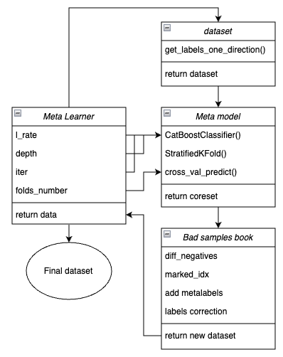
Figure 1. Schematic representation of meta_learner() function

It should be recalled that the meta learner is a transmission gear between the initial data and the final model. It takes on the main burden of effective preprocessing by creating meta labels through a meta model. The uniqueness of the function I developed lies in the fact that it creates cleared and well-prepared datasets, due to which robust models and trading systems are occur.

Function input parameters:

• l_rate (learning rate)  is the gradient step for the meta model or CatBoost classifier. It is set in the range from {0.01, 0.5}. The algorithm is sensitive to this parameter.
• depth is responsible for the depth of the decision trees that are built on each iteration of the CatBoost classifier training. Recommended range of values is {1, 6}
• iter is the number of training iterations, it is recommended in the range {5, 25}
• folds_number is the number of folds for cross-validation. Usually, {5, 15} folds are enough.

The mechanism of function operation:

• A dataset with features and labels is created. The get_labels_one_direction() function described earlier is used as a sampler.
• A meta learner with the specified parameters is trained on this data in cross-validation mode using the StratifiedKFold() function. The function divides the training data into several folds, subject to the balance of classes. A meta model is trained on each fold, and then all predictions are saved. This is necessary in order to obtain an unbiased estimate of model errors on training data. These predictions will be used for comparison with the original labels.

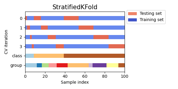
Fig. 2. A scheme for dividing data into folds using the StratifiedKFold() function

• A separate coreset dataset is created, which records both the original and predicted labels through cross-validation. 
• A separate variable diff_negatives is created that stores binary flags of matches between the original and predicted labels.
• A book of bad samples B_S_B (Bad Samples Book) is created. It records the time indexes of those dataset rows for which predictions did not match the original labels.
• Unique indexes of incorrectly predicted examples for all folds are determined.
• An additional column 'meta_labels' is created in the original dataset and all observations are assigned '1' (you can trade).
• For all examples that were incorrectly predicted during the cross-validation process, a '0' is assigned in the 'meta_labels' column (do not trade).
• For all incorrectly predicted samples, in the 'labels' column, which contains labels for the main model, '0' is also assigned (do not trade).
• The function returns a modified dataset.

A more reliable causal inference

In the previous section, we discussed the basic meta learner, which example makes it easier to explain the basic concept. In this section, we somewhat complicate the approach and look directly at the process of causal inference itself. I adapted the causal inference function from the linked article for the case of unidirectional trading. It is more advanced and has more flexible functionality.

def meta_learners(models_number: int, iterations: int, depth: int, bad_samples_fraction: float):
    dataset = get_labels_one_direction(get_features(get_prices()),
                                       markup=hyper_params['markup'],
                                       min=1,
                                       max=15,
                                       direction=hyper_params['direction'])
    data = dataset[(dataset.index < hyper_params['forward']) & (dataset.index > hyper_params['backward'])].copy()

    X = data[data.columns[1:-2]]
    y = data['labels']

    BAD_WAIT = pd.DatetimeIndex([])
    BAD_TRADE = pd.DatetimeIndex([])

    for i in range(models_number):
        X_train, X_val, y_train, y_val = train_test_split(
            X, y, train_size = 0.5, test_size = 0.5, shuffle = True)
        
        # learn debias model with train and validation subsets
        meta_m = CatBoostClassifier(iterations = iterations,
                                depth = depth,
                                custom_loss = ['Accuracy'],
                                eval_metric = 'Accuracy',
                                verbose = False,
                                use_best_model = True)
        
        meta_m.fit(X_train, y_train, eval_set = (X_val, y_val), plot = False)
        
        coreset = X.copy()
        coreset['labels'] = y
        coreset['labels_pred'] = meta_m.predict_proba(X)[:, 1]
        coreset['labels_pred'] = coreset['labels_pred'].apply(lambda x: 0 if x < 0.5 else 1)
        
        # add bad samples of this iteration (bad labels indices)
        coreset_w = coreset[coreset['labels']==0]
        coreset_t = coreset[coreset['labels']==1]

        diff_negatives_w = coreset_w['labels'] != coreset_w['labels_pred']
        diff_negatives_t = coreset_t['labels'] != coreset_t['labels_pred']
        BAD_WAIT = BAD_WAIT.append(diff_negatives_w[diff_negatives_w == True].index)
        BAD_TRADE = BAD_TRADE.append(diff_negatives_t[diff_negatives_t == True].index)

    to_mark_w = BAD_WAIT.value_counts()
    to_mark_t = BAD_TRADE.value_counts()
    marked_idx_w = to_mark_w[to_mark_w > to_mark_w.mean() * bad_samples_fraction].index
    marked_idx_t = to_mark_t[to_mark_t > to_mark_t.mean() * bad_samples_fraction].index

    data['meta_labels'] = 1.0
    data.loc[data.index.isin(marked_idx_w), 'meta_labels'] = 0.0
    data.loc[data.index.isin(marked_idx_t), 'meta_labels'] = 0.0
    data.loc[data.index.isin(marked_idx_t), 'labels'] = 0.0

    return data[data.columns[:]]

Below is a scheme of meta learner function in the form of key blocks responsible for various functions.

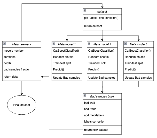
Figure 3. Schematic representation of meta_learners() function

A distinctive feature of this function is that it has several "heads" of meta models that are trained on random subsamples of the original dataset, which are selected using the bootstrap method with a return. This method enables to perform multiple generation of subsamples from the source dataset. Statistical and probabilistic characteristics can be estimated on this set of pseudo-samples.

For example, we are interested in the average value of how well this particular example, taken from the general population, is predicted if we trained models on different subsamples of this population. This will give us a less biased view of each of the aggregate examples, which can then be labeled as bad or good examples with a higher degree of confidence.

Function input parameters:

• models number is the number of meta models that are used in the algorithm. Recommended range of values {5, 100}
• iterations  is the number of training iterations for each model. Recommended range of values {15, 35}
• depth   is the depth of the decision trees that are built on each iteration of the CatBoost classifier training. Recommended range of values is {1, 6}
• bad samples fraction  is the number of samples that will be marked as "bad". Recommended range of values is{0.4, 0.9}

The mechanism of function operation:

• A dataset is being created with features and labels of a given trade direction.
• In the loop, each of the meta models is trained on randomly selected training and validation data using the bootstrap method.

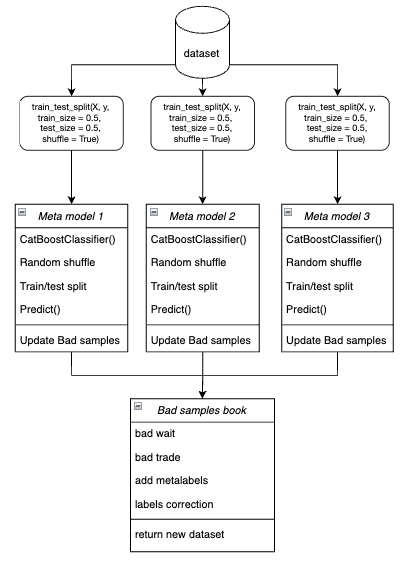
Figure 4. Schematic representation of bootstrap sampling

• For each model, its predictions are compared with the true labels. Indexes of incorrectly classified cases are saved in the book of bad samples.
• The average number of incorrectly predicted indexes across all passes is determined.
• The indexes that have the largest number of incorrectly predicted labels, and which exceed the average multiplied by the threshold, are added to the "meta_labels" column as zeros (trade ban).
• The 'labels' are set to zero according to the same principle.

The philosophy behind using the meta learner for unidirectional trading:

• The meta learner code solves the problem of filtering "bad" signals in a marked-up dataset.
• Simplifying the classification task. Features are optimized for only one type of patterns (for example, trend continuation).
• Even with the balance of classes (50% of buys/ 50% of sells), asymmetry remains in the trend. Trend buys have more stable patterns, while countertrend sells are often associated with noise events (corrections, false reversals) that are difficult to predict.
• For sells in a growing trend, most signals are initially false (False positives), which leads to classification errors. Accordingly, in the case of bidirectional trading, buy and sell trades are of different nature and cannot be compared.
• In a unidirectional system, errors are associated only with false entries into a trend trade (for example, entry before correction). The meta learner effectively finds such cases, as they have clear signs (for example, overbought). In a bidirectional system, errors include false buys and sells, which may have similar patterns. The meta learner cannot reliably separate the "noise" from real signals, as the features for buys/sells are mixed. 
• In a unidirectional system, the model focuses on one type of non-stationarity (for example, trend strengthening) and features adapt to the current market phase.
• In a bidirectional system, there are two non-stationarities (trend + correction), which requires twice as much data and is more difficult to generalize. 

Result:

• The classification task is simplified — it is enough to correctly predict one class instead of two.
• Noise is reduced — the final meta model filters only one type of error.
• Cross-validation improves because stratification functions correctly.
• Trend non—stationarity is taken into account - the model adapts to only one market phase.

An important feature of meta learners:

Meta learners should not be confused with the final meta model, which is trained on the labels prepared by meta learners. Meta learners are not final models and are used only at the preprocessing phase. Any binary classification algorithms can be used as basic learners, including logistic regression, neural networks, “tree-based" models, and other exotic models. In addition, regression models can be used with minor code modifications, which is beyond the scope of this article and can be discussed in subsequent ones. For convenience, I use CatBoost binary classifier, because I'm used to working with it.

Features related to learning attributes

It has already been mentioned above that trading in one direction simplifies the task of classification. Features are optimized for only one type of patterns (for example, buys), so there is no need for symmetrical features. Symmetrical features can be called both the initial time series with different time lags, the values of which correspond to buy and sell trades, as well as various derivatives (price increments) and other oscillators. Non-symmetrical features include volatility in different time windows, since it reflects only the rate of change in prices, but not their direction. This project will use volatility with different windows set in the 'periods' variable.

Here is the complete code that implements the creation of features:

def get_features(data: pd.DataFrame) -> pd.DataFrame:
    pFixed = data.copy()
    pFixedC = data.copy()
    count = 0

    for i in hyper_params['periods']:
        pFixed[str(count)] = pFixedC.rolling(i).std()
        count += 1
    return pFixed.dropna()

And the periods of sliding windows for calculating such features are specified in the dictionary. They can be changed arbitrarily and look at model performance.

hyper_params = {
    'periods': [i for i in range(5, 300, 30)],
}

In this example, we create 10 features, the first of which has a period of 5, and each subsequent period increases by 30, and so on to 300:

>>> [i for i in range(5, 300, 30)]
[5, 35, 65, 95, 125, 155, 185, 215, 245, 275]

Training and testing of unidirectional models

hyper_params = {
    'symbol': 'XAUUSD_H1',
    'export_path': '/drive_c/Program Files/MetaTrader 5/MQL5/Include/Mean reversion/',
    'model_number': 0,
    'markup': 0.25,
    'stop_loss':  10.0000,
    'take_profit': 5.0000,
    'direction': 'buy',
    'periods': [i for i in range(5, 300, 30)],
    'backward': datetime(2020, 1, 1),
    'forward': datetime(2024, 1, 1),
    'full forward': datetime(2026, 1, 1),
}

models = []
for i in range(10):
    print('Learn ' + str(i) + ' model')
    models.append(fit_final_models(meta_learner(5, 15, 3, 0.1)))
    # models.append(fit_final_models(meta_learners(25, 15, 3, 0.8)))

First, we will test the first meta learner, and the second one will be commented out. Сhoose the direction of buy trading as the preferred one, because gold is on a growing trend right now. The training will take place from the beginning of 2020 until 2024. While the test period was selected from the beginning of 2024 to April 1, 2025.

The meta learner has the following settings:

• 5 folds for cross-validation
• 15 training iterations for the CatBoost algorithm
• the depth of the tree for each iteration is 3
• learning rate is 0.1

This is what the best model looks like in the strategy tester for the 'buy' direction:

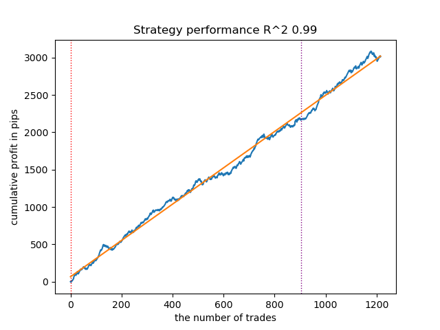
Figure 5. Results of testing features of the meta_learner() function in the buy direction

For comparison, this is what the best model for the "sell" direction looks like:

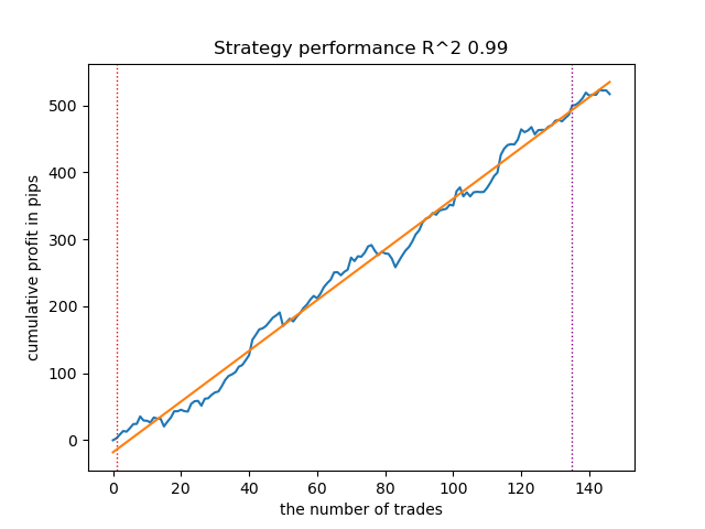
Figure 6. Results of testing features of the meta_learner() function in the sell direction

The algorithm has learned to predict trades both in the buy direction and in the sell direction. But there were much fewer sell trades, which is natural for a growing trending market. The meta-model acted quite effectively even without selecting its hyperparameters, which is reflected in both the training and forward-testing areas.

Now, discuss a more advanced meta learner. Perform similar manipulations for the meta_learners() function. Let's uncomment it and comment on the previous one:

models = []
for i in range(10):
    print('Learn ' + str(i) + ' model')
    # models.append(fit_final_models(meta_learner(5, 15, 3, 0.1)))
    models.append(fit_final_models(meta_learners(25, 15, 3, 0.8)))

The meta learner has the following settings:

• 25 "heads" or meta-models
• 15 training iterations for the CatBoost algorithm for each of the models
• the depth of the tree for each iteration is 3
• 0.8 for the "bad_samples_fraction" parameter, which determines the percentage of bad samples left in the training dataset. 0.1 will correspond to very strong filtering, and 0.9 will filter out few bad samples.

This is what the best model looks like in the strategy tester for the 'buy' direction:

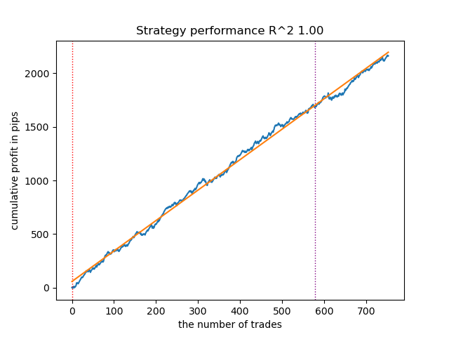
Figure 7. Results of testing features of the meta_learners() function in the buy direction

For comparison, this is what the best model for the "sell" direction looks like:

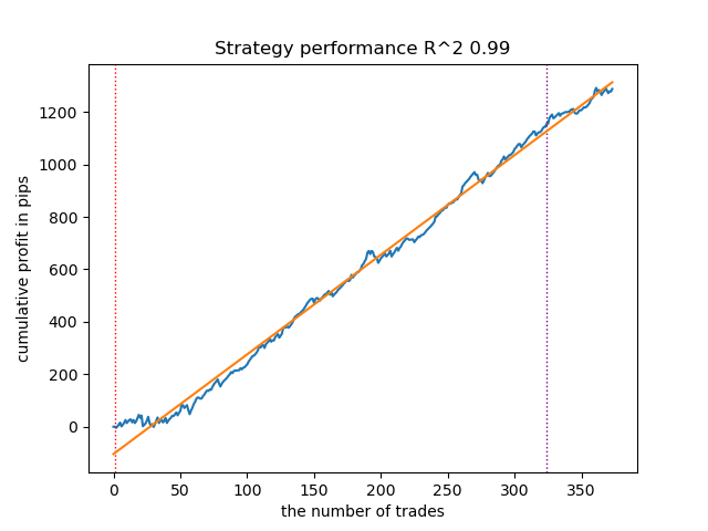
Figure 8. Results of testing features of the meta_learners() function in the sell direction

A more advanced meta learner function showed more beautiful curves. The balance for buy and sell trades was saved. Obviously, the best strategy is a buy strategy. After the models are trained and the best model is selected, you can export them to the Meta Trader 5 terminal. You can use both strategies, but since the strategy of opening short positions is less effective, we choose only the strategy for long positions.

Below is a table of dependencies of learning outcomes on advanced meta learner parameters:

Parameter name:	Impact on filtering quality:
models_number: int	The more "heads" or meta-models there are, the less biased the assessment of bad samples is.  The size of the training dataset affects the choice of the number of models. The longer the history is, the more models you may need. It is necessary to experiment, varying this parameter in the range from 5 to 100.
iterations: int	Greatly affects the filtration rate. The more iterations of training each meta learner, the slower the rate is. Small values can lead to under-training, which can lead to stronger filtering and a small number of trades at the output. It is recommended to set it in the range from 5 to 50.
depth: int	The depth of the tree is set in the range from 1 to 6. At each iteration, the algorithm completes the tree of a given depth. I use a depth of 3, but you can experiment with this parameter.
bad_samples_fraction: float	It affects the final selection of bad samples and the number of trades. 0.9 corresponds to "soft" filtering and a large number of trades at the output. 0.5 corresponds to "hard" filtering and, as a result, a small number of trades at the output.

Finishing touches: exporting models and creating a trading advisor

The models are exported in exactly the same way that is used in other articles. To do this, select the model you like from the sorted list of models and call the export function.

models.sort(key=lambda x: x[0])
data = get_features(get_prices())
test_model_one_direction(data,
        models[-1][1:],
        hyper_params['stop_loss'],
        hyper_params['take_profit'],
        hyper_params['forward'],
        hyper_params['backward'],
        hyper_params['markup'],
        hyper_params['direction'],
        plt=True)

export_model_to_ONNX(models[-1], 0)

The logic of the trading bot has been changed so that it will only trade in one direction, depending on the model you exported.

input bool direction = true;           //True = Buy, False = Sell

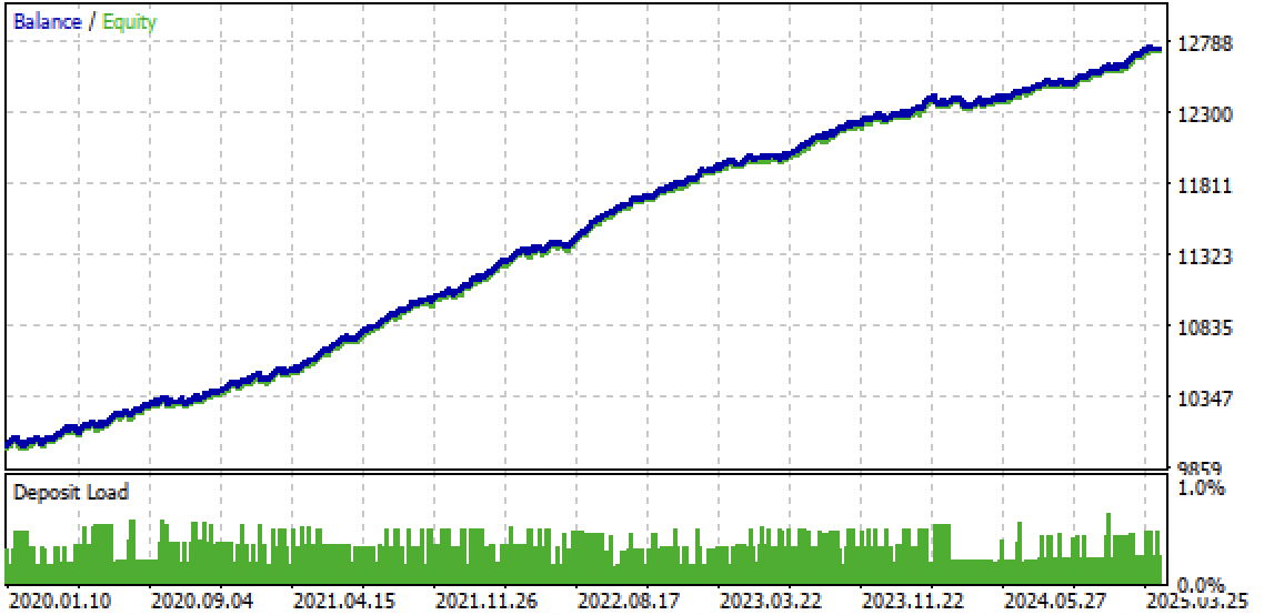
Fig. 9. Testing the bot in the Meta Trader 5 terminal

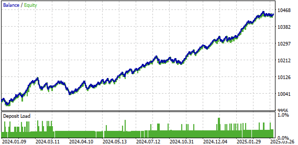
Fig. 10. Testing only on the forward period from the beginning of 2024

Conclusion

The idea of unidirectional strategies using machine learning seemed interesting to me, so I conducted a number of experiments, including the approach proposed in this article. It is not the only possible one, but it copes well with the task. Such trend-dependent strategies can show good performance if the trend continues. Therefore, it is important to monitor global trend changes and adjust such systems to the current market situation.

 Python files.zip archive contains the following files for development in Python:

File name	Description
causal one direction.py	The main script for learning models
labeling_lib.py	Updated module with trade markers
tester_lib.py	Updated custom tester for machine learning-based strategies
XAUUSD_H1.csv	The quotation file exported from the MetaTrader 5 terminal

 MQL5 files.zip archive contains files for MetaTrader 5:

File name	Description
one direction.ex5	Compiled bot from this article
one direction.mq5	The source of the bot from the article
folder Include//Trend following	Location of the ONNX models and the header file for connecting to the bot.