基于机器学习构建均值回归策略

MetaTrader 5 — 交易 | 27 一月 2026, 14:31

[删除]

概述

本文提出了另一种基于机器学习构建交易系统的原创方法。在先前的文章中，我已经探讨了将聚类分析应用于因果推断问题的方法。而在本文中，聚类分析将被用于将金融时间序列划分为具有独特特性的多种模式，随后将针对每种模式构建并测试交易系统。

此外，我们还将探讨几种为均值回归策略标注样本的方法，并在被认为走势平稳的欧元兑英镑（EURGBP）货币对上测试这些方法，这意味着这些策略应能完全适用于该货币对。

本文将指导您如何在Python中训练各种机器学习模型，并将它们转换为MetaTrader 5交易终端的交易系统。

准备必要的软件包

模型训练将在Python中进行，因此请确保已经安装好以下软件包：

import math
import pandas as pd
import pickle
from datetime import datetime
from catboost import CatBoostClassifier

from sklearn.model_selection import train_test_split
from sklearn.cluster import KMeans

from bots.botlibs.labeling_lib import *
from bots.botlibs.tester_lib import tester
from bots.botlibs.export_lib import export_model_to_ONNX

最后三个模块是我编写的。将它们附在文章末尾处。每个模块可能还会导入其他软件包，如Scipy、Numpy、Sklearn、Numba等，这些软件包也需要安装。这些软件包广为人知且公开可用，因此安装过程应该不会有问题。

如果您的Python环境是全新的，那么以下是您需要安装的软件包列表：

pip install numpy
pip install pandas
pip install scipy
pip install scikit-learn
pip install catboost
pip install numba

根据您的开发环境以及文章末尾所附库文件的位置，您可能还需要使用绝对导入路径来导入这些库。

代码设计时并未完全依赖Python解释器的版本或特定软件包，但推荐使用最新的稳定版本。

如何为均值回归策略标注样本？

让我们回顾一下之前文章中我们是如何标注标签的。我们创建了一个循环，其中每次单独交易的持续时间被随机设定，例如从1到15根K线。然后，根据自虚拟交易开仓以来经过的K线数量内市场是上涨还是下跌，我们放置一个买入或卖出标记。该函数返回一个包含特征和标注标签的数据结构，此时数据集已完全准备好，可用于后续的机器学习模型训练。

def get_labels(dataset, markup, min = 1, max = 15) -> pd.DataFrame:
    labels = []
    for i in range(dataset.shape[0]-max):
        rand = random.randint(min, max)
        curr_pr = dataset['close'].iloc[i]
        future_pr = dataset['close'].iloc[i + rand]

        if (future_pr + markup) < curr_pr:
            labels.append(1.0)
        elif (future_pr - markup) > curr_pr:
            labels.append(0.0)
        else:
            labels.append(2.0)
        
    dataset = dataset.iloc[:len(labels)].copy()
    dataset['labels'] = labels
    dataset = dataset.dropna()
    dataset = dataset.drop(
        dataset[dataset.labels == 2.0].index)
    return dataset

但这种标注方式存在一个显著缺陷——它是随机的。通过这种方式标注数据，我们并未对机器学习模型应逼近何种模式提出任何明确要求。因此，这种标注和训练的结果在很大程度上也将是随机的。我们曾尝试通过多次暴力训练（即大量随机尝试）并使算法架构更加复杂来解决这一问题，但标注本身仍然缺乏实际意义。由于采用随机抽样，只有部分模型能够通过样本外（OOS）测试。

在本文中，我提出了一种基于原始时间序列过滤的全新交易标注方法。让我们通过一个例子来了解一下这种标注方式。

图例1. 萨维茨基-戈拉（Savitzky-Golay）滤波器及分位数带的展示

图1展示了萨维茨基-戈拉滤波器的平滑曲线，以及20分位数和80分位数带，这在一定程度上让人联想到布林带。萨维茨基-戈拉滤波器与普通移动平均线的主要区别在于，它不会相对于价格产生滞后。由于这一特性，该滤波器能很好地平滑价格，而剩余的“噪声”则是相对于均值（即滤波器本身的值）的偏差，这些偏差可用于制定均值回归策略。当上下分位数带交叉时，会形成卖出或买入信号。如果价格上穿上线，则为卖出信号。如果价格下穿下线，则为买入信号。

萨维茨基-戈拉滤波器是一种数字滤波器，用于平滑数据并抑制噪声，同时保留重要的信号特征，如峰值和趋势。它由亚伯拉罕·萨维茨基（Abraham Savitzky）和马塞尔·J·E·戈拉（Marcel J. Е. Golay）于1964年提出。该滤波器在信号处理和数据分析领域得到广泛应用。

萨维茨基-戈拉滤波器通过使用最小二乘法，用低次（二次、三次或四次）多项式对数据进行局部近似来工作。对于每个数据点，选择一个邻域（窗口），并用多项式对该窗口内的数据进行近似。近似后，窗口中心的值被替换为使用多项式计算出的值。这使我们能够在保持信号形式的同时平滑噪声。

以下是构建滤波器并进行可视化评估的代码。

def plot_close_filter_quantiles(dataset, rolling=200, quantiles=[0.2, 0.8], polyorder=3):
    # Calculate smoothed prices
    smoothed = savgol_filter(dataset['close'], 
                            window_length=rolling, 
                            polyorder=polyorder)
    
    # Calculate difference between prices and filter
    lvl = dataset['close'] - smoothed
    
    # Get quantile values
    q_low, q_high = lvl.quantile(quantiles).tolist()
    
    # Calculate bands based on quantiles
    upper_band = smoothed + q_high  # Upper band
    lower_band = smoothed + q_low   # Lower band
    
    # Create plot
    plt.figure(figsize=(14, 7))
    plt.plot(dataset.index, dataset['close'], label='Close Prices', color='blue', alpha=0.5)
    plt.plot(dataset.index, smoothed, label=f'Smoothed (window={rolling})', color='orange', linewidth=2)
    plt.plot(dataset.index, upper_band, label=f'Upper Quantile ({quantiles[1]*100:.0f}%)', 
             color='green', linestyle='--')
    plt.plot(dataset.index, lower_band, label=f'Lower Quantile ({quantiles[0]*100:.0f}%)', 
             color='red', linestyle='--')
    
    # Configure display
    plt.title('Price and Filter with Quantile Bands')
    plt.xlabel('Date')
    plt.ylabel('Price')
    plt.legend()
    plt.grid(True)
    plt.show()

因此，若将此滤波器直接应用于非平稳时间序列的在线处理将是错误的，因为最新值可能会被重新计算（即出现未来数据泄漏问题），但它非常适合用于对现有数据进行交易标注。

让我们编写代码，利用萨维茨基-戈拉滤波器实现训练样本的标注。标注函数（以及其他类似函数）位于labeling_lib.py这个Python模块中，后续我们将把它导入到项目中。

@njit
def calculate_labels_filter(close, lvl, q):
    labels = np.empty(len(close), dtype=np.float64)
    for i in range(len(close)):
        curr_lvl = lvl[i]

        if curr_lvl > q[1]:
            labels[i] = 1.0
        elif curr_lvl < q[0]:
            labels[i] = 0.0
        else:
            labels[i] = 2.0
    return labels

def get_labels_filter(dataset, rolling=200, quantiles=[.45, .55], polyorder=3) -> pd.DataFrame:
    """
    Generates labels for a financial dataset based on price deviation from a Savitzky-Golay filter.

    This function applies a Savitzky-Golay filter to the closing prices to generate a smoothed
    price trend. It then calculates trading signals (buy/sell) based on the deviation of the 
    actual price from this smoothed trend. Buy signals are generated when the price is 
    significantly below the smoothed trend, anticipating a potential price reversal. 

    Args:
        dataset (pd.DataFrame): DataFrame containing financial data with a 'close' column.
        rolling (int, optional): Window size for the Savitzky-Golay filter. Defaults to 200.
        quantiles (list, optional): Quantiles to define the "reversion zone". Defaults to [.45, .55].
        polyorder (int, optional): Polynomial order for the Savitzky-Golay filter. Defaults to 3.

    Returns:
        pd.DataFrame: The original DataFrame with a new 'labels' column and filtered rows:
                       - 'labels' column: 
                            - 0: Buy
                            - 1: Sell
                       - Rows where 'labels' is 2 (no signal) are removed.
                       - Rows with missing values (NaN) are removed.
                       - The temporary 'lvl' column is removed. 
    """

    # Calculate smoothed prices using the Savitzky-Golay filter
    smoothed_prices = savgol_filter(dataset['close'].values, window_length=rolling, polyorder=polyorder)
    
    # Calculate the difference between the actual closing prices and the smoothed prices
    diff = dataset['close'] - smoothed_prices
    dataset['lvl'] = diff  # Add the difference as a new column 'lvl' to the DataFrame
    
    # Remove any rows with NaN values 
    dataset = dataset.dropna()
    
    # Calculate the quantiles of the 'lvl' column (price deviation)
    q = dataset['lvl'].quantile(quantiles).to_list() 

    # Extract the closing prices and the calculated 'lvl' values as NumPy arrays
    close = dataset['close'].values
    lvl = dataset['lvl'].values
    
    # Calculate buy/sell labels using the 'calculate_labels_filter' function 
    labels = calculate_labels_filter(close, lvl, q) 

    # Trim the dataset to match the length of the calculated labels
    dataset = dataset.iloc[:len(labels)].copy()
    
    # Add the calculated labels as a new 'labels' column to the DataFrame
    dataset['labels'] = labels
    
    # Remove any rows with NaN values
    dataset = dataset.dropna()
    
    # Remove rows where the 'labels' column has a value of 2.0 (no signals)
    dataset = dataset.drop(dataset[dataset.labels == 2.0].index)
    
    # Return the modified DataFrame with the 'lvl' column removed
    return dataset.drop(columns=['lvl'])

为加速标注过程，我们使用了前一篇文章中介绍的Numba包。

get_labels_filter()函数接收包含价格和基于价格构建特征的原始数据集、滤波器近似窗口的长度、上下分位数的边界值以及多项式阶数作为输入。该函数的输出是在原始数据集中添加买入或卖出标签，这些标签随后可用于训练数据集。

历史循环在名为calc_labels_filter的独立函数中实现，该函数使用Numba包进行高性能计算。

这种标注方式具有以下特点：

并非所有标注的交易都能盈利，因为价格在穿越分位数带后，并不总是会向相反方向变动。这可能导致样本被错误地标注为买入或卖出。
从理论上讲，这一缺点可通过标注的均匀性和非随机性得到弥补。因此，错误标注的样本可被视为训练误差或整个交易系统的误差，这有助于减少最终模型的过拟合现象。

交易标注逻辑的完整描述如下：

calculate_labels_filter函数

输入数据：

close：收盘价数组
lvl：价格相对于平滑趋势的偏差数组
q：定义信号区域的分位数数组

逻辑如下：

1. 初始化：创建与收盘价数组close长度相同的空labels数组，用于存储交易信号。

2. 遍历价格：针对每个收盘价close[i]及其对应的偏差值lvl[i]：

卖出信号：若偏差值lvl[i]超过上分位数q[1]，表明价格显著高于平滑趋势，生成卖出信号（labels[i] = 1.0）。
买入信号：若偏差值lvl[i]低于下分位数q[0]，表明价格显著低于平滑趋势，生成买入信号（labels[i] = 0.0）。
无信号：其他情况（偏差值位于分位数之间），不生成信号（labels[i] = 2.0）。

3. 返回结果：返回包含交易信号的labels数组。

get_labels_filter函数

输入数据：

dataset：包含金融数据的DataFrame，其中包含close列（收盘价）。
rolling：用于平滑的Savitzky-Golay滤波器的窗口大小。
quantiles：用于确定信号区域的分位数。
polyorder：Savitzky-Golay平滑多项式的阶数。

逻辑如下：

1. 价格平滑：

对收盘价（dataset['close']）应用Savitzky-Golay滤波器，计算平滑后的价格smoothed_prices。

2. 计算偏差：

计算实际收盘价与平滑价格之间的差值（diff）。
将差值作为新列lvl添加到DataFrame中。

3. 移除缺失值：

从DataFrame中移除包含缺失值（NaN）的行。

4. 计算分位数：

计算lvl列的分位数，用于确定信号区域。

5. 信号计算：

调用calculate_labels_filter函数，传入收盘价、偏差值和分位数。
获取包含交易信号的labels数组。

6. DataFrame处理：

将DataFrame截断至与labels数组相同的长度。
将labels数组作为新列labels添加到DataFrame中。
移除labels等于2.0的行（无信号）。
移除临时列lvl。

7. 返回结果：返回修改后的DataFrame，其中labels列包含买入和卖出信号。

我们将上述标注方法视为标准方法，通过它展示了均值回归策略标注的基本原理。这是一种可行的方法，可以投入使用。我们可以对其进行泛化和修改，以适应多个滤波器，并考虑偏离均值的方差变化。以下是实现这些更改的get_labels_multiple_filters函数。

@njit
def calc_labels_multiple_filters(close, lvls, qs):
    labels = np.empty(len(close), dtype=np.float64)
    for i in range(len(close)):
        label_found = False
        
        for j in range(len(lvls)):
            curr_lvl = lvls[j][i]
            curr_q_low = qs[j][0][i]
            curr_q_high = qs[j][1][i]
            
            if curr_lvl > curr_q_high:
                labels[i] = 1.0
                label_found = True
                break
            elif curr_lvl < curr_q_low:
                labels[i] = 0.0
                label_found = True
                break
                
        if not label_found:
            labels[i] = 2.0
            
    return labels

def get_labels_multiple_filters(dataset, 
                              rolling_periods=[200, 400, 600], 
                              quantiles=[.45, .55], 
                              window=100,
                              polyorder=3) -> pd.DataFrame:
    """
    Generates trading signals (buy/sell) based on price deviation from multiple 
    smoothed price trends calculated using a Savitzky-Golay filter with different
    rolling periods and rolling quantiles. 

    This function applies a Savitzky-Golay filter to the closing prices for each 
    specified 'rolling_period'. It then calculates the price deviation from these
    smoothed trends and determines dynamic "reversion zones" using rolling quantiles.
    Buy signals are generated when the price is within these reversion zones 
    across multiple timeframes.

    Args:
        dataset (pd.DataFrame): DataFrame containing financial data with a 'close' column.
        rolling_periods (list, optional): List of rolling window sizes for the Savitzky-Golay filter. 
                                           Defaults to [200, 400, 600].
        quantiles (list, optional): Quantiles to define the "reversion zone". Defaults to [.05, .95].
        window (int, optional): Window size for calculating rolling quantiles. Defaults to 100.
        polyorder (int, optional): Polynomial order for the Savitzky-Golay filter. Defaults to 3.

    Returns:
        pd.DataFrame: The original DataFrame with a new 'labels' column and filtered rows:
                       - 'labels' column: 
                            - 0: Buy
                            - 1: Sell
                       - Rows where 'labels' is 2 (no signal) are removed.
                       - Rows with missing values (NaN) are removed. 
    """
    
    # Create a copy of the dataset to avoid modifying the original
    dataset = dataset.copy()
    
    # Lists to store price deviation levels and quantiles for each rolling period
    all_levels = []
    all_quantiles = []
    
    # Calculate smoothed price trends and rolling quantiles for each rolling period
    for rolling in rolling_periods:
        # Calculate smoothed prices using the Savitzky-Golay filter
        smoothed_prices = savgol_filter(dataset['close'].values, 
                                      window_length=rolling, 
                                      polyorder=polyorder)
        # Calculate the price deviation from the smoothed prices
        diff = dataset['close'] - smoothed_prices
        
        # Create a temporary DataFrame to calculate rolling quantiles
        temp_df = pd.DataFrame({'diff': diff})
        
        # Calculate rolling quantiles for the price deviation
        q_low = temp_df['diff'].rolling(window=window).quantile(quantiles[0])
        q_high = temp_df['diff'].rolling(window=window).quantile(quantiles[1])
        
        # Store the price deviation and quantiles for the current rolling period
        all_levels.append(diff)
        all_quantiles.append([q_low.values, q_high.values])
    
    # Convert lists to NumPy arrays for faster calculations (potentially using Numba)
    lvls_array = np.array(all_levels)
    qs_array = np.array(all_quantiles)
    
    # Calculate buy/sell labels using the 'calc_labels_multiple_filters' function 
    labels = calc_labels_multiple_filters(dataset['close'].values, lvls_array, qs_array)
    
    # Add the calculated labels to the DataFrame
    dataset['labels'] = labels
    
    # Remove rows with NaN values and no signals (labels == 2.0)
    dataset = dataset.dropna()
    dataset = dataset.drop(dataset[dataset.labels == 2.0].index)
    
    # Return the DataFrame with the new 'labels' column
    return dataset

该函数可接受任意数量的Savitzky-Golay平滑参数。由于标注将涉及多个不同周期的滤波器，这一点会带来额外的益处。只要至少有一个滤波器在分位边界处触发“偏离均值”条件，即可形成信号。

这使我们能够构建分层次的标记结构。例如，先检查高通滤波器，再检查带通滤波器，最后检查低通滤波器。低通信号被视为更可靠，因此如果低通产生信号，则将覆盖之前的所有信号。但是如果低通滤波器未生成交易信号，则交易仍将基于先前滤波器生成的信号进行标注。这样既增加了标注样本数量，又允许使用更高的输入阈值（分位数），因为多滤波器组合提高了“至少一个信号出现”的概率。

分位计算现在采用可配置周期的滑动窗口，从而把“偏离均值的方差变化”纳入考虑，使信号更加精准。

最后，我们还可以考虑非对称交易场景，假设报价均值存在偏斜，可能需要采用不同平滑周期的滤波器来分别标记买入和卖出订单。该方法在get_labels_filter_bidirectional函数中实现。

@njit
def calc_labels_bidirectional(close, lvl1, lvl2, q1, q2):
    labels = np.empty(len(close), dtype=np.float64)
    for i in range(len(close)):
        curr_lvl1 = lvl1[i]
        curr_lvl2 = lvl2[i]

        if curr_lvl1 > q1[1]:
            labels[i] = 1.0
        elif curr_lvl2 < q2[0]:
            labels[i] = 0.0
        else:
            labels[i] = 2.0
    return labels

def get_labels_filter_bidirectional(dataset, rolling1=200, rolling2=200, quantiles=[.45, .55], polyorder=3) -> pd.DataFrame:
    """
    Generates trading labels based on price deviation from two Savitzky-Golay filters applied
    in opposite directions (forward and reversed) to the closing price data.

    This function calculates trading signals (buy/sell) based on the price's 
    position relative to smoothed price trends generated by two Savitzky-Golay filters 
    with potentially different window sizes (`rolling1`, `rolling2`). 

    Args:
        dataset (pd.DataFrame): DataFrame containing financial data with a 'close' column.
        rolling1 (int, optional): Window size for the first Savitzky-Golay filter. Defaults to 200.
        rolling2 (int, optional): Window size for the second Savitzky-Golay filter. Defaults to 200.
        quantiles (list, optional): Quantiles to define the "reversion zones". Defaults to [.45, .55].
        polyorder (int, optional): Polynomial order for both Savitzky-Golay filters. Defaults to 3.

    Returns:
        pd.DataFrame: The original DataFrame with a new 'labels' column and filtered rows:
                       - 'labels' column: 
                            - 0: Buy
                            - 1: Sell
                       - Rows where 'labels' is 2 (no signal) are removed.
                       - Rows with missing values (NaN) are removed.
                       - Temporary 'lvl1' and 'lvl2' columns are removed.
    """

    # Apply the first Savitzky-Golay filter (forward direction)
    smoothed_prices = savgol_filter(dataset['close'].values, window_length=rolling1, polyorder=polyorder)
    
    # Apply the second Savitzky-Golay filter (could be in reverse direction if rolling2 is negative)
    smoothed_prices2 = savgol_filter(dataset['close'].values, window_length=rolling2, polyorder=polyorder)

    # Calculate price deviations from both smoothed price series
    diff1 = dataset['close'] - smoothed_prices
    diff2 = dataset['close'] - smoothed_prices2

    # Add price deviations as new columns to the DataFrame
    dataset['lvl1'] = diff1
    dataset['lvl2'] = diff2
    
    # Remove rows with NaN values 
    dataset = dataset.dropna()

    # Calculate quantiles for the "reversion zones" for both price deviation series
    q1 = dataset['lvl1'].quantile(quantiles).to_list()
    q2 = dataset['lvl2'].quantile(quantiles).to_list()

    # Extract relevant data for label calculation
    close = dataset['close'].values
    lvl1 = dataset['lvl1'].values
    lvl2 = dataset['lvl2'].values
    
    # Calculate buy/sell labels using the 'calc_labels_bidirectional' function
    labels = calc_labels_bidirectional(close, lvl1, lvl2, q1, q2)

    # Process the dataset and labels
    dataset = dataset.iloc[:len(labels)].copy()
    dataset['labels'] = labels
    dataset = dataset.dropna()
    dataset = dataset.drop(dataset[dataset.labels == 2.0].index) # Remove bad signals (if any)
    
    # Return the DataFrame with temporary columns removed
    return dataset.drop(columns=['lvl1', 'lvl2'])

该函数接受两个平滑周期参数rolling1和rolling2，分别对应卖出和买入交易的标记。通过调整这些参数，可以尝试在新数据上实现更优的标注效果和泛化能力。例如，如果某货币对呈上升趋势且更适宜开立买入仓位，则可延长用于标记卖出交易的rolling1窗口长度，从而减少卖出信号数量，或仅在真正出现强趋势反转时生成卖出信号。对于买入交易，可缩短rolling2窗口长度，使买入信号数量多于卖出信号。

基于盈利交易限制与滤波器选择的标注方法

正如前文所提及，提出的交易标记方法允许存在被标记但明显无利可图的交易。这并非缺陷，而是设计特性。

我们可添加校验机制，确保仅标记盈利交易。如果需使资金曲线更接近理想直线（无显著回撤），此方法将颇具价值。

此外，当前仅使用单一Savitzky-Golay滤波器，但为提升多样性，拟增加简单移动平均线和样条曲线作为滤波器。

让我们来探讨此类交易采样器的实现方案。我们将以get_labels_mean_reversion函数为基础，该函数支持盈利性限制与滤波器选择功能。

@njit
def calculate_labels_mean_reversion(close, lvl, markup, min_l, max_l, q):
    labels = np.empty(len(close) - max_l, dtype=np.float64)
    for i in range(len(close) - max_l):
        rand = random.randint(min_l, max_l)
        curr_pr = close[i]
        curr_lvl = lvl[i]
        future_pr = close[i + rand]

        if curr_lvl > q[1] and (future_pr + markup) < curr_pr:
            labels[i] = 1.0
        elif curr_lvl < q[0] and (future_pr - markup) > curr_pr:
            labels[i] = 0.0
        else:
            labels[i] = 2.0
    return labels

def get_labels_mean_reversion(dataset, markup, min_l=1, max_l=15, rolling=0.5, quantiles=[.45, .55], method='spline', shift=0) -> pd.DataFrame:
    """
    Generates labels for a financial dataset based on mean reversion principles.

    This function calculates trading signals (buy/sell) based on the deviation of
    the price from a chosen moving average or smoothing method. It identifies
    potential buy opportunities when the price deviates significantly below its 
    smoothed trend, anticipating a reversion to the mean.

    Args:
        dataset (pd.DataFrame): DataFrame containing financial data with a 'close' column.
        markup (float): The percentage markup used to determine buy signals.
        min_l (int, optional): Minimum number of consecutive days the markup must hold. Defaults to 1.
        max_l (int, optional): Maximum number of consecutive days the markup is considered. Defaults to 15.
        rolling (float, optional): Rolling window size for smoothing/averaging. 
                                     If method='spline', this controls the spline smoothing factor.
                                     Defaults to 0.5.
        quantiles (list, optional): Quantiles to define the "reversion zone". Defaults to [.45, .55].
        method (str, optional): Method for calculating the price deviation:
                                 - 'mean': Deviation from the rolling mean.
                                 - 'spline': Deviation from a smoothed spline.
                                 - 'savgol': Deviation from a Savitzky-Golay filter.
                                 Defaults to 'spline'.
        shift (int, optional): Shift the smoothed price data forward (positive) or backward (negative).
                                 Useful for creating a lag/lead effect. Defaults to 0.

    Returns:
        pd.DataFrame: The original DataFrame with a new 'labels' column and filtered rows:
                       - 'labels' column: 
                            - 0: Buy
                            - 1: Sell
                       - Rows where 'labels' is 2 (no signal) are removed.
                       - Rows with missing values (NaN) are removed.
                       - The temporary 'lvl' column is removed. 
    """

    # Calculate the price deviation ('lvl') based on the chosen method
    if method == 'mean':
        dataset['lvl'] = (dataset['close'] - dataset['close'].rolling(rolling).mean())
    elif method == 'spline':
        x = np.array(range(dataset.shape[0]))
        y = dataset['close'].values
        spl = UnivariateSpline(x, y, k=3, s=rolling) 
        yHat = spl(np.linspace(min(x), max(x), num=x.shape[0]))
        yHat_shifted = np.roll(yHat, shift=shift) # Apply the shift
        dataset['lvl'] = dataset['close'] - yHat_shifted
        dataset = dataset.dropna()  # Remove NaN values potentially introduced by spline/shift
    elif method == 'savgol':
        smoothed_prices = savgol_filter(dataset['close'].values, window_length=int(rolling), polyorder=3)
        dataset['lvl'] = dataset['close'] - smoothed_prices

    dataset = dataset.dropna()  # Remove NaN values before proceeding
    q = dataset['lvl'].quantile(quantiles).to_list()  # Calculate quantiles for the 'reversion zone'

    # Prepare data for label calculation
    close = dataset['close'].values
    lvl = dataset['lvl'].values
    
    # Calculate buy/sell labels 
    labels = calculate_labels_mean_reversion(close, lvl, markup, min_l, max_l, q) 

    # Process the dataset and labels
    dataset = dataset.iloc[:len(labels)].copy()
    dataset['labels'] = labels
    dataset = dataset.dropna()
    dataset = dataset.drop(dataset[dataset.labels == 2.0].index)  # Remove sell signals (if any)
    return dataset.drop(columns=['lvl'])  # Remove the temporary 'lvl' column

我采用了本章节开头讨论并在先前文章中使用过的get_labels函数代码，作为检查交易盈利性及构建基础逻辑的依据。根据这一原则，首先对经过滤波器标记的交易进行筛选。仅保留未来指定步数内盈利的交易；未达盈利条件的交易则标记为2.0并从数据集中移除。此外，我还新增了两种滤波器：移动平均线和样条曲线。

虽然移动平均线在交易领域广为人知，但样条曲线的构建方法对部分读者而言可能较为陌生，因此需要特别说明。

样条曲线是一种灵活的函数逼近工具。与用单一复杂多项式拟合整个函数不同，样条曲线将定义域划分为多个区间，并在每个区间上单独构建多项式。这些多项式在区间边界处平滑衔接，形成连续且光滑的曲线。

尽管样条曲线类型多样，但其构建均遵循类似原理：

定义域划分：将函数原始定义区间通过节点分割为多个子区间。
多项式阶数选择：确定每个子区间拟合多项式的阶数。
多项式构建：在每个子区间上构建通过该区间数据点的指定阶数多项式。
平滑性保证：通过调整多项式系数比率，确保样条曲线在区间边界处的平滑性。这样通常要求相邻多项式的函数值及其导数在节点处保持一致。

在金融时间序列分析中，样条曲线具有以下应用价值：

数据插值与平滑：样条曲线可以平滑数据噪声，并估算缺失测量点的时间序列值。
趋势模拟：分离长期趋势与短期波动，构建数据趋势模型。
预测分析：部分样条曲线类型可用于时间序列未来值预测。
导数估算：通过样条曲线估算时间序列的导数，能够辅助分析价格变化速率。

在本研究中，我们将采用与Savitzky-Golay滤波器相同的处理方式，分别通过样条曲线和移动平均线对时间序列进行平滑处理。我们随后可以单独使用各滤波器进行交易标记，通过对比结果选择最优方案以适应特定场景需求。

图例2. 样条滤波器及其分位数带展示

图2展示了样条滤波器的平滑曲线，以及20%和80%分位数带。样条滤波器与Savitzky-Golay滤波器的主要区别在于：它通过分段线性或非线性函数对序列进行平滑处理，具体取决于平滑因子s（建议取值范围为0.1至1）和多项式阶数（通常设为1至3）。通过调整这些参数，可以直观评估不同平滑效果。代码中默认固定多项式阶数k=3，但用户也可根据需要修改。

样条滤波器的构建与可视化代码示例如下：

import pandas as pd
from scipy.interpolate import UnivariateSpline
import matplotlib.pyplot as plt

def plot_close_filter_quantiles(dataset, rolling=200, quantiles=[0.2, 0.8]):
    """
    Plots close prices with spline smoothing and quantile bands.

    Args:
        dataset (pd.DataFrame): DataFrame with 'close' column and datetime index.
        rolling (int, optional): Rolling window size for spline smoothing. 
                                  Defaults to 200.
        quantiles (list, optional): Quantiles for band calculation. 
                                     Defaults to [0.2, 0.8].
        s (float, optional): Smoothing factor for UnivariateSpline. 
                             Adjusts the spline stiffness. Defaults to 1000.
    """
    
    # Create spline smoothing
    # Convert datetime index to numerical values (Unix timestamps)
    numerical_index = pd.to_numeric(dataset.index)
    
    # Create spline smoothing using the numerical index
    spline = UnivariateSpline(numerical_index, dataset['close'], k=3, s=rolling)  
    smoothed = spline(numerical_index)
    
    # Calculate difference between prices and filter
    lvl = dataset['close'] - smoothed
    
    # Get quantile values
    q_low, q_high = lvl.quantile(quantiles).tolist()
    
    # Calculate bands based on quantiles
    upper_band = smoothed + q_high
    lower_band = smoothed + q_low
    
    # Create plot
    plt.figure(figsize=(14, 7))
    plt.plot(dataset.index, dataset['close'], label='Close Prices', color='blue', alpha=0.5)
    plt.plot(dataset.index, smoothed, label=f'Spline Smoothed (s={rolling})', color='orange', linewidth=2)
    plt.plot(dataset.index, upper_band, label=f'Upper Quantile ({quantiles[1]*100:.0f}%)', 
             color='green', linestyle='--')
    plt.plot(dataset.index, lower_band, label=f'Lower Quantile ({quantiles[0]*100:.0f}%)', 
             color='red', linestyle='--')
    
    # Configure display
    plt.title('Price and Spline with Quantile Bands')
    plt.xlabel('Date')
    plt.ylabel('Price')
    plt.legend()
    plt.grid(True)
    plt.show()

以下是关于calculate_labels_mean_reversion函数的详细说明，旨在帮助全面理解交易信号标注代码的核心逻辑。

calculate_labels_mean_reversion函数：

输入数据：

close：收盘价数组
lvl：与平滑序列相比的价格偏离数组
markup：以百分比表示
min_l：测试条件所需的最少K线数量
max_l：测试条件所需的最多K线数量
定义信号区域的分位数数组

逻辑如下：

1. 初始化：创建一个长度为len(close) - max_l的空数组labels，用于存储交易信号。缩短长度是为了预留未来价格数据的空间。

2. 遍历价格序列：对每个收盘价close[i]（索引i从0到len(close) - max_l - 1）执行以下操作：

在min_l和max_l之间定义一个随机数rand。
获取当前价格curr_pr、当前偏离值curr_lvl以及rand根K线后的未来价格future_pr。
卖出信号：如果curr_lvl高于上分位数 (q[1])，且考虑markup后的未来价格future_pr低于当前价格，则设置labels[i] = 1.0。
买入信号：如果curr_lvl低于下分位数 (q[0])，且future_pr - markup高于当前价格，则设置labels[i] = 0.0。
无信号：其余情况设置labels[i] = 2.0。

3. 返回结果：返回包含交易信号的labels数组。

get_labels_mean_reversion函数：

输入数据：

dataset：包含“收盘价”列的金融数据的DataFrame
markup：以百分比表示
min_l：测试条件所需的最少K线数量
max_l：测试条件所需的最多K线数量
rolling：平滑参数（窗口大小或比率）
quantiles：用于确定信号区域的分位数。
method：平滑方法（'mean'、'spline'、'savgol'）
shift：平滑序列的平移

逻辑如下：

1. 偏离值计算：根据选定的method计算价格序列（收盘价）相对于平滑曲线的偏离值lvl：

mean：相对于移动平均线的偏离值
spline：相对于样条平滑曲线的偏离值
savgol：相对于Savitzky-Golay滤波平滑曲线的偏离值

2. 缺失值处理：从dataset中移除包含缺失值（NaN）的行。

3. 分位数计算：计算偏离值lvl的q分位数。

4. 数据准备：从dataset中提取收盘价数组close和偏离值数组lvl。

5. 信号计算：

调用calculate_labels_mean_reversion函数，传入准备好的数据，生成包含交易信号的labels数组。

6. DataFrame处理：

将dataset截断至与labels长度一致。
将labels作为新列labels添加到dataset。
移除dataset中包含NaN的行。
移除labels等于2.0的行（无信号）。
移除lvl列。

7. 返回结果：返回修改后的dataset，其中labels列包含买入（0.0）和卖出（1.0）信号。

为了增加多样性，让我们实现一个相同的采样器版本，它将检查多个不同周期滤波器的条件，而非单一周期。只有当所有滤波器的条件都被满足，且它们方向一致（全部为买入或全部为卖出），并且交易在未来n根K线内是盈利的，才满足标注条件；否则，忽略该样本并将其从训练集中移除。

@njit
def calculate_labels_mean_reversion_multi(close_data, lvl_data, q, markup, min_l, max_l, windows):
    labels = []
    for i in range(len(close_data) - max_l):
        rand = random.randint(min_l, max_l)
        curr_pr = close_data[i]
        future_pr = close_data[i + rand]

        buy_condition = True
        sell_condition = True
        qq = 0
        for rolling in windows:
            curr_lvl = lvl_data[i, qq]            
            if not (curr_lvl >= q[qq][1]):
                sell_condition = False
            if not (curr_lvl <= q[qq][0]):
                buy_condition = False
            qq+=1
    
        if sell_condition and (future_pr + markup) < curr_pr:
            labels.append(1.0)
        elif buy_condition and (future_pr - markup) > curr_pr:
            labels.append(0.0)
        else:
            labels.append(2.0)
    return labels

def get_labels_mean_reversion_multi(dataset, markup, min_l=1, max_l=15, windows=[0.2, 0.3, 0.5], quantiles=[.45, .55]):
    """
    Generates labels for a financial dataset based on mean reversion 
    principles using multiple smoothing windows.

    This function calculates trading signals (buy/sell) based on the deviation 
    of the price from smoothed price trends calculated using multiple spline 
    smoothing factors (windows). It identifies potential buy opportunities when 
    the price deviates significantly below its smoothed trends across multiple
    timeframes.

    Args:
        dataset (pd.DataFrame): DataFrame containing financial data with a 'close' column.
        markup (float): The percentage markup used to determine buy signals.
        min_l (int, optional): Minimum number of consecutive days the markup must hold. Defaults to 1.
        max_l (int, optional): Maximum number of consecutive days the markup is considered. Defaults to 15.
        windows (list, optional): List of smoothing factors (rolling window equivalents) 
                                   for spline calculations. Defaults to [0.2, 0.3, 0.5].
        quantiles (list, optional): Quantiles to define the "reversion zone". Defaults to [.45, .55].

    Returns:
        pd.DataFrame: The original DataFrame with a new 'labels' column and filtered rows:
                       - 'labels' column: 
                            - 0: Buy
                            - 1: Sell
                       - Rows where 'labels' is 2 (sell signal) are removed.
                       - Rows with missing values (NaN) are removed. 
    """

    q = []  # Initialize an empty list to store quantiles for each window
    lvl_data = np.empty((dataset.shape[0], len(windows)))  # Initialize a 2D array to store price deviation data

    # Calculate price deviation from smoothed trends for each window
    for i, rolling in enumerate(windows):
        x = np.array(range(dataset.shape[0]))  # Create an array of x-values (time index)
        y = dataset['close'].values  # Extract closing prices
        spl = UnivariateSpline(x, y, k=3, s=rolling)  # Create a spline smoothing function
        yHat = spl(np.linspace(min(x), max(x), num=x.shape[0]))  # Generate smoothed price data
        lvl_data[:, i] = dataset['close'] - yHat  # Calculate price deviation from smoothed prices
        q.append(np.quantile(lvl_data[:, i], quantiles).tolist())  # Calculate and store quantiles

    dataset = dataset.dropna()  # Remove NaN values before proceeding

    close_data = dataset['close'].values  # Extract closing prices 

    # Calculate buy/hold labels using multiple price deviation series
    labels = calculate_labels_mean_reversion_multi(close_data, lvl_data, q, markup, min_l, max_l, windows)

    # Process the dataset and labels
    dataset = dataset.iloc[:len(labels)].copy()  # Trim the dataset to match label length
    dataset['labels'] = labels  # Add the calculated labels as a new column
    dataset = dataset.dropna()  # Remove rows with NaN values
    dataset = dataset.drop(dataset[dataset.labels == 2.0].index)  # Remove sell signals (if any)
    
    return dataset

最后，我们再编写一个均值回归交易信号标注函数，该函数基于滑动窗口周期计算分位数，而非在整个历史观测期内统一计算。该方法能有效平滑价格偏离均值时因波动率变化导致的信号噪声。

@njit
def calculate_labels_mean_reversion_v(close_data, lvl_data, volatility_group, quantile_groups, markup, min_l, max_l):
    labels = []
    for i in range(len(close_data) - max_l):
        rand = random.randint(min_l, max_l)
        curr_pr = close_data[i]
        curr_lvl = lvl_data[i]
        curr_vol_group = volatility_group[i]
        future_pr = close_data[i + rand]

        q = quantile_groups[curr_vol_group]

        if curr_lvl > q[1] and (future_pr + markup) < curr_pr:
            labels.append(1.0)
        elif curr_lvl < q[0] and (future_pr - markup) > curr_pr:
            labels.append(0.0)
        else:
            labels.append(2.0)
    return labels

def get_labels_mean_reversion_v(dataset, markup, min_l=1, max_l=15, rolling=0.5, quantiles=[.45, .55], method='spline', shift=1, volatility_window=20) -> pd.DataFrame:
    """
    Generates trading labels based on mean reversion principles, incorporating
    volatility-based adjustments to identify buy opportunities.

    This function calculates trading signals (buy/sell), taking into account the 
    volatility of the asset. It groups the data into volatility bands and calculates 
    quantiles for each band. This allows for more dynamic "reversion zones" that 
    adjust to changing market conditions.

    Args:
        dataset (pd.DataFrame): DataFrame containing financial data with a 'close' column.
        markup (float): The percentage markup used to determine buy signals.
        min_l (int, optional): Minimum number of consecutive days the markup must hold. Defaults to 1.
        max_l (int, optional): Maximum number of consecutive days the markup is considered. Defaults to 15.
        rolling (float, optional): Rolling window size or spline smoothing factor (see 'method'). 
                                     Defaults to 0.5.
        quantiles (list, optional): Quantiles to define the "reversion zone". Defaults to [.45, .55].
        method (str, optional): Method for calculating the price deviation:
                                 - 'mean': Deviation from the rolling mean.
                                 - 'spline': Deviation from a smoothed spline.
                                 - 'savgol': Deviation from a Savitzky-Golay filter.
                                 Defaults to 'spline'.
        shift (int, optional): Shift the smoothed price data (lag/lead effect). Defaults to 1.
        volatility_window (int, optional): Window size for calculating volatility. Defaults to 20.

    Returns:
        pd.DataFrame: The original DataFrame with a new 'labels' column and filtered rows:
                       - 'labels' column: 
                            - 0: Buy
                            - 1: Sell
                       - Rows where 'labels' is 2 (no signal) are removed.
                       - Rows with missing values (NaN) are removed.
                       - Temporary 'lvl', 'volatility', 'volatility_group' columns are removed.
    """

    # Calculate Volatility
    dataset['volatility'] = dataset['close'].pct_change().rolling(window=volatility_window).std()
    
    # Divide into 20 groups by volatility 
    dataset['volatility_group'] = pd.qcut(dataset['volatility'], q=20, labels=False)
    
    # Calculate price deviation ('lvl') based on the chosen method
    if method == 'mean':
        dataset['lvl'] = (dataset['close'] - dataset['close'].rolling(rolling).mean())
    elif method == 'spline':
        x = np.array(range(dataset.shape[0]))
        y = dataset['close'].values
        spl = UnivariateSpline(x, y, k=3, s=rolling)
        yHat = spl(np.linspace(min(x), max(x), num=x.shape[0]))
        yHat_shifted = np.roll(yHat, shift=shift) # Apply the shift 
        dataset['lvl'] = dataset['close'] - yHat_shifted
        dataset = dataset.dropna() 
    elif method == 'savgol':
        smoothed_prices = savgol_filter(dataset['close'].values, window_length=rolling, polyorder=5)
        dataset['lvl'] = dataset['close'] - smoothed_prices

    dataset = dataset.dropna()
    
    # Calculate quantiles for each volatility group
    quantile_groups = {}
    for group in range(20):
        group_data = dataset[dataset['volatility_group'] == group]['lvl']
        quantile_groups[group] = group_data.quantile(quantiles).to_list()
    
    # Prepare data for label calculation (potentially using Numba)
    close_data = dataset['close'].values
    lvl_data = dataset['lvl'].values
    volatility_group = dataset['volatility_group'].values

    # Calculate buy/sell labels 
    labels = calculate_labels_mean_reversion_v(close_data, lvl_data, volatility_group, quantile_groups, markup, min_l, max_l)
    
    # Process dataset and labels
    dataset = dataset.iloc[:len(labels)].copy()
    dataset['labels'] = labels
    dataset = dataset.dropna()
    dataset = dataset.drop(dataset[dataset.labels == 2.0].index) # Remove sell signals
    
    # Remove temporary columns and return
    return dataset.drop(columns=['lvl', 'volatility', 'volatility_group'])

至此，我们已经拥有了一系列可供实验的交易信号标记方法。这些方法可以自由组合，开发全新的信号生成策略。

以下是从labeling_lib.py库中导出的完整交易信号采样器清单。在此基础上，您可以根据自己对市场模式的理解程度，以及最终想要实现的策略类型，来修改旧采样器或创建全新的采样器。该模块还包含其他自定义交易采样器，但它们与均值回归策略无关，因此本文不作描述。

# FILTERING BASED LABELING W/O RESTRICTIONS
def get_labels_filter(dataset, rolling=200, quantiles=[.45, .55], polyorder=3) -> pd.DataFrame
def get_labels_multiple_filters(dataset, rolling_periods=[200, 400, 600], quantiles=[.45, .55], window=100, polyorder=3) -> pd.DataFrame
def get_labels_filter_bidirectional(dataset, rolling1=200, rolling2=200, quantiles=[.45, .55], polyorder=3) -> pd.DataFrame:

# MEAN REVERSION WITH RESTRICTIONS BASED LABELING
def get_labels_mean_reversion(dataset, markup, min_l=1, max_l=15, rolling=0.5, quantiles=[.45, .55], method='spline', shift=0) -> pd.DataFrame
def get_labels_mean_reversion_multi(dataset, markup, min_l=1, max_l=15, windows=[0.2, 0.3, 0.5], quantiles=[.45, .55]) -> pd.DataFrame
def get_labels_mean_reversion_v(dataset, markup, min_l=1, max_l=15, rolling=0.5, quantiles=[.45, .55], method='spline', shift=1, volatility_window=20) -> pd.DataFrame:

现在是时候进入本文的第二部分——市场状态聚类，并将聚类方法与均值回归策略结合，构建完整的交易系统。

为何需要聚类？聚类的目标是什么？

在开始聚类前，我们需要明确其必要性。想象一张价格图表：包含趋势、震荡、高波动/低波动期、各类形态等特征。也就是说，价格图表并非一成不变，不存在完全相同的模式。甚至可以说，不同时间段可能存在截然不同的模式，且这些模式会随时间消失或演变。

聚类让您能够根据某些特征把原始时间序列划分成若干“状态”，每个状态都描述了相似的观测结果。这样能让构建交易系统的任务变得更简单，因为训练将在更同质、更相似的数据上进行。至少，您可以如此设想。自然而然地，交易系统不再在整个历史周期上运行，而只在由不同时间点组成、且这些时间点的值落在给定聚类内的选定片段上运行。

聚类之后，只需对被选中的样本进行标注（即赋予唯一类别标签），即可构建最终模型。如果一个聚类包含的是相似观测值的同质数据，那么它的标注应该会更同质，进而更具可预测性。您可以取多个数据聚类，分别对它们进行标注，然后在每个聚类的数据上训练机器学习模型，并在训练集和测试集上进行测试。如果找到一个能让模型很好地学习（即泛化并预测新数据）的聚类，那么就认为构建交易系统的任务已经基本完成。

对金融时间序列进行聚类以识别市场模式

在阅读本节之前，建议熟悉先前的文章中描述的各种聚类算法类型。该文章还提供了不同聚类算法的对比表及其测试结果。本文选用传统的k-means聚类算法，因其速度最快、效率最高。

在通过get_features函数创建特征的阶段，我们需要提前在数据集中预留“用于聚类的特征”。我建议从以下三种基础方案入手。如果您有其他能充分刻画市场状态的特征，尽管使用。只需在特征生成函数中添加其计算逻辑，并在命名时包含"meta_feature"字符串，以便与主特征区分开来。

def get_features(data: pd.DataFrame) -> pd.DataFrame:
    pFixed = data.copy()
    pFixedC = data.copy()
    count = 0

    for i in hyper_params['periods']:
        pFixed[str(count)] = pFixedC.rolling(i).mean()
        count += 1
    
    for i in hyper_params['periods_meta']:
        pFixed[str(count)+'meta_feature'] = pFixedC.rolling(i).skew()
        count += 1

    # for i in hyper_params['periods_meta']:
    #     pFixed[str(count)+'meta_feature'] = pFixedC.rolling(i).std()
    #     count += 1

    # for i in hyper_params['periods_meta']:
    #     pFixed[str(count)+'meta_feature'] = pFixedC - pFixedC.rolling(i).mean()
    #     count += 1

    return pFixed.dropna()

在第一轮循环中，计算periods列表中的所有特征。这些是训练主模型（预测买入或卖出）的核心特征，本文默认使用不同周期的简单移动平均线。

在第二轮循环中，计算periods_meta列表中的特征。这些特征正是专门用于市场状态聚类的要素。默认情况下，聚类将基于滑动窗口内价格报价的偏度进行计算。被注释掉的字段对应于基于滑动窗口标准差或价格增量计算的特征。特征的选择通过经验性枚举多选项来完成。实验表明，基于偏度（非对称性）的聚类能较好地区分数据，因此本文将采用该方法。

分布的偏度（或非对称性）是描述数据分布相对于均值不对称程度的特征。用来衡量分布与对称性（如正态分布）的偏离程度。通过偏度系数（skewness）量化。偏度聚类通过识别具有相似分布特征的数据组，可有效划分不同的市场状态。例如，正偏度可能对应高波动剧烈行情（如危机期），负偏度可能对应低波动震荡行情。

特征构建完成后，将最终数据集传入聚类函数。新增一列"clusters"，用于存放所属聚类编号。

def clustering(dataset, n_clusters: int) -> pd.DataFrame:
    data = dataset[(dataset.index < hyper_params['forward']) & (dataset.index > hyper_params['backward'])].copy()
    meta_X = data.loc[:, data.columns.str.contains('meta_feature')]
    data['clusters'] = KMeans(n_clusters=n_clusters).fit(meta_X).labels_
    return data

为避免“数据窥探”，算法会根据设定日期对数据进行前后截断，确保聚类仅使用模型训练阶段实际可用的数据。代码中还通过特征列名中的meta_feature关键词，筛选出用于聚类的特征。

所有算法超参数均存储于字典中，其数据将用于创建特征、选择训练周期等。

hyper_params = {
    'symbol': 'EURGBP_H1',
    'export_path': '/Users/dmitrievsky/Library/Containers/com.isaacmarovitz.Whisky/Bottles/54CFA88F-36A3-47F7-915A-D09B24E89192/drive_c/Program Files/MetaTrader 5/MQL5/Include/Mean reversion/',
    # 'export_path': '/Users/dmitrievsky/Library/Containers/com.isaacmarovitz.Whisky/Bottles/54CFA88F-36A3-47F7-915A-D09B24E89192/drive_c/Program Files (x86)/RoboForex MT4 Terminal/MQL4/Include/',
    'model_number': 0,
    'markup': 0.00010,
    'stop_loss':  0.02000,
    'take_profit': 0.00200,
    'periods': [i for i in range(5, 300, 30)],
    'periods_meta': [10],
    'backward': datetime(2000, 1, 1),
    'forward': datetime(2021, 1, 1),
    'n_clusters': 10,
    'rolling': 200,
}

在磁盘内存储交易品种报价数据的文件名
将训练好的模型导出至MetaTrader 5终端的#include目录
在需要导出多个模型时使用模型ID区分
标记应考虑平均点差和佣金，以点为单位。为了更精确地标注交易订单，并支持后续的历史数据回测。
快速自定义测试器支持的止损
止盈
主特征计算周期列表列表中的每个元素对应一个独立特征的周期参数。元素越多，生成的特征越多。
参与聚类的特征周期列表。
模型训练的起始日期
模型训练的结束日期
数据将被划分的聚类数量（市场状态数）
滤波平滑的滑动窗口参数

接下来，我们将整合所有内容，查看模型训练的主循环，并分析预处理与训练阶段的完整流程。

# LEARNING LOOP
dataset = get_features(get_prices())
models = []
for i in range(1):
    data = clustering(dataset, n_clusters=hyper_params['n_clusters'])
    sorted_clusters = data['clusters'].unique()
    sorted_clusters.sort()
    for clust in sorted_clusters:
        clustered_data = data[data['clusters'] == clust].copy()
        if len(clustered_data) < 500:
            print('too few samples: {}'.format(len(clustered_data)))
            continue
    
        clustered_data = get_labels_filter(clustered_data, 
                                           rolling=hyper_params['rolling'],
                                           quantiles=[0.45, 0.55],
                                           polyorder=3
                                            )

        print(f'Iteration: {i}, Cluster: {clust}')
        clustered_data = clustered_data.drop(['close', 'clusters'], axis=1)

        meta_data = data.copy()
        meta_data['clusters'] = meta_data['clusters'].apply(lambda x: 1 if x == clust else 0)
        models.append(fit_final_models(clustered_data, meta_data.drop(['close'], axis=1)))

首先，创建一个包含价格和特征的数据集。特征生成方法已在前文中描述过。接着，初始化一个空列表models，用于存储训练好的模型。随后，我们需要确定训练循环的迭代次数。默认执行1次迭代。如果需训练多个模型，可在range()迭代器中指定数量。

对原始数据集进行聚类，为每个样本分配聚类编号。如果超参数中设定n_clusters=10，则数据将被划分为10个聚类。实验表明，10个聚类能较好地覆盖市场状态，当然，该参数可以根据需求调整。

随后，确定最终聚类数量，按升序排列聚类编号，并逐号筛选对应行。我们忽略样本过少的聚类（<500 条），确保训练充分。

下一步，对当前聚类调用交易标注函数。在本例中，我沿用文章最初的get_labels_filter。标注完成后，数据被拆成两份数据集。第一份主数据集包含核心特征与标签，第二份基础数据集包含用于聚类的meta特征及0/1标签。1表示数据对应的所选聚类，0表示数据对应所选聚类以外的其他聚类。归根结底，我们希望交易系统只在特定的市场模式下进行交易。

因此，第一个模型将学习预测交易方向，第二个模型将学习何时可以开仓、何时应该观望。

让我们看一下fit_final_models函数本身，该函数为两个最终模型接收两份数据集，并在此基础上训练CatBoost算法。

def fit_final_models(clustered, meta) -> list:
    # features for model\meta models. We learn main model only on filtered labels 
    X, X_meta = clustered[clustered.columns[:-1]], meta[meta.columns[:-1]]
    X = X.loc[:, ~X.columns.str.contains('meta_feature')]
    X_meta = X_meta.loc[:, X_meta.columns.str.contains('meta_feature')]
    
    # labels for model\meta models
    y = clustered['labels']
    y_meta = meta['clusters']
    
    y = y.astype('int16')
    y_meta = y_meta.astype('int16')

    # train\test split
    train_X, test_X, train_y, test_y = train_test_split(
        X, y, train_size=0.7, test_size=0.3, shuffle=True)
    
    train_X_m, test_X_m, train_y_m, test_y_m = train_test_split(
        X_meta, y_meta, train_size=0.7, test_size=0.3, shuffle=True)


    # learn main model with train and validation subsets
    model = CatBoostClassifier(iterations=1000,
                               custom_loss=['Accuracy'],
                               eval_metric='Accuracy',
                               verbose=False,
                               use_best_model=False,
                               task_type='CPU',
                               thread_count=-1)
    model.fit(train_X, train_y, eval_set=(test_X, test_y),
              early_stopping_rounds=30, plot=False)
    
    # learn meta model with train and validation subsets
    meta_model = CatBoostClassifier(iterations=500,
                                    custom_loss=['F1'],
                                    eval_metric='F1',
                                    verbose=False,
                                    use_best_model=True,
                                    task_type='CPU',
                                    thread_count=-1)
    meta_model.fit(train_X_m, train_y_m, eval_set=(test_X_m, test_y_m),
              early_stopping_rounds=25, plot=False)

    
    R2 = test_model([model, meta_model], hyper_params['stop_loss'], hyper_params['take_profit'])
    if math.isnan(R2):
        R2 = -1.0
        print('R2 is fixed to -1.0')
    print('R2: ' + str(R2))

    return [R2, model, meta_model]

训练阶段：

1. 数据准备：

从clustered和meta输入数据框中提取特征（X, X_meta）和标签（y, y_meta）。
将标签数据类型转换为int16。这是无缝转换为ONNX格式所必需的。
使用train_test_split将数据划分为训练集和测试集。

2. 主模型训练：

根据给定超参数创建CatBoostClassifier对象。
使用训练数据（train_X, train_y）训练模型，并利用验证集（test_X, test_y）进行早停。

3. 基础模型训练：

根据给定的超参数为基础模型创建另一个CatBoostClassifier对象。
使用与主模型类似的方式训练基础模型，使用对应的训练和测试数据。

4. 模型评估：

将训练好的模型（model, meta_model）连同止损（stop_loss）和止盈（take_profit）参数传入test_model函数进行性能评估。
返回的R²值作为模型性能指标。

5. 处理R²值并返回结果：

如果R²为NaN，则替换为-1.0。
在屏幕上显示R²值。
函数返回包含R²和训练好的模型（model, meta_model）列表。

对于每个聚类，生成两个训练好的分类模型，可直接用于最终可视化测试结果并且导出至MetaTrader 5终端。每次训练迭代会生成与超参数中指定聚类数量相等的模型对。聚类数量乘以迭代次数，可以大致了解总共会生成多少对模型。例如，如果指定10个聚类和10次迭代，那么将输出100对模型，未通过样本量过滤的聚类除外。

模型训练与测试：算法测试

为了便于使用算法，推荐在交互式的Python环境中逐行运行代码。这样便于我们调整超参数或尝试不同的采样器。或者，我们可以将所有代码转换为.ipynb格式，以便通过笔记本电脑在IPython中运行。如果您需要运行完整的脚本，请提前编辑参数配置。

建议对每个标注函数运行10次迭代测试。其余参数保持脚本默认值。

启动训练循环后，会显示每次迭代中每个数据聚类的训练结果。

R2: 0.9815970951474068
Iteration: 9, Cluster: 5
R2: 0.9914890771969395
Iteration: 9, Cluster: 6
R2: 0.9450681335265942
Iteration: 9, Cluster: 7
R2: 0.9631330369697314
Iteration: 9, Cluster: 8
R2: 0.9680380185183347
Iteration: 9, Cluster: 9
R2: 0.8203651933893291

随后，我们可以将所有结果按R²值升序排列，从中筛选出性能最优者。此外，我们还可以直观地评估测试器中的平衡曲线。

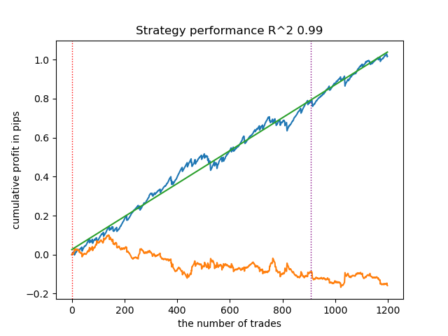
models.sort(key=lambda x: x[0])
test_model(models[-1][1:], hyper_params['stop_loss'], hyper_params['take_profit'], plt=True)

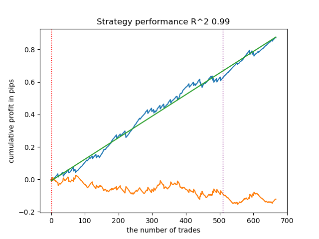
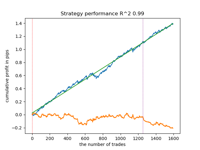
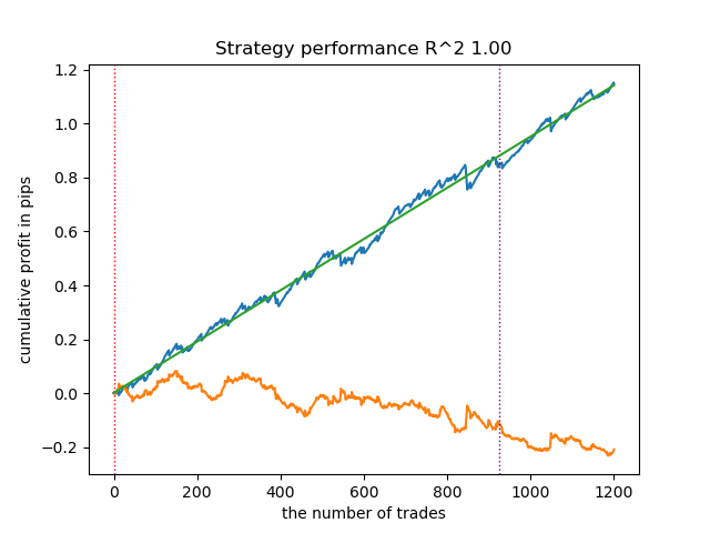
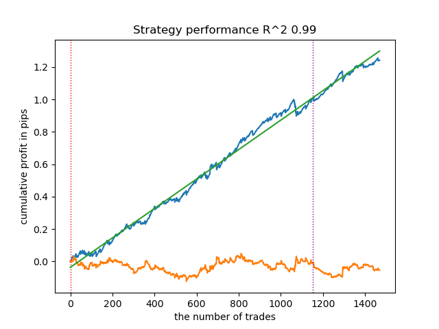
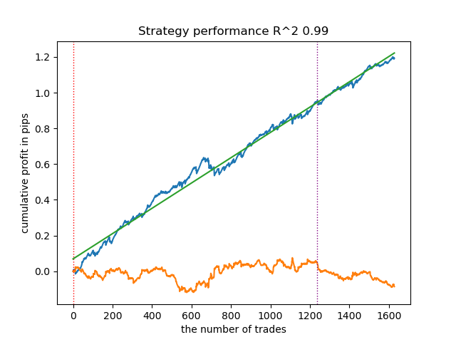
高亮部分表示将测试倒数第一个模型（即R²值最高的模型）。如果需测试倒数第二个模型，需要将索引设置为-2，依此类推。测试器将显示这些：策略资金曲线（蓝色）、货币对价格走势（橙色）和划分训练期与新数据（测试期）的垂直分界线所有模型的训练区间均为2010年初至2021年初（由超参数指定）。您可以根据需要自行调整训练和测试区间。本文中所有模型的测试区间为2021年初至2025年初。

测试不同交易采样器

get_labels_filter(dataset, rolling=200, quantiles=[.45, .55], polyorder=3)

以下为get_labels_filter信号生成器的最优表现：

该基础信号生成器呈现良好的交易标注效果，所有模型在新数据上均实现盈利。让我们对剩余信号生成器重复相同测试流程，并对比结果。

get_labels_multiple_filters(dataset,rolling_periods=[50,100,200],quantiles=[.45,.55],window=100,polyorder=3)

基于该信号标记数据训练的模型，其交易次数通常较基准模型显著提升。本文未进行调优实验，否则篇幅将过长。

get_labels_filter_bidirectional(dataset, rolling1=50, rolling2=200, quantiles=[.45, .55], polyorder=3)

该非对称信号标记在新数据上同样展现了有效性。通过分别为买入和卖出交易设置不同的平滑参数，可以进一步优化结果。

现在，让我们转向严格盈利交易限制的信号标记。显然，之前的信号标记即使在训练期内也未能生成平滑的资金曲线，但它们对市场模式的捕捉能力较强。现在，我们尝试从训练数据中剔除亏损交易，观察效果变化。

get_labels_mean_reversion(dataset, markup, min_l=1, max_l=15, rolling=0.5, quantiles=[.45, .55], method='spline', shift=0)

测试中使用了样条曲线和固定平滑因子（0.5）。文章未对Savitzky-Golay滤波器和简单移动平均线进行测试。然而，由此可见通过交易盈利性限制，资金曲线平滑度显著提升。

get_labels_mean_reversion_multi(dataset, markup, min_l=1, max_l=15, windows=[0.2, 0.3, 0.5], quantiles=[.45, .55])

该采样器能生成高质量样本，使模型在新数据上持续盈利。

get_labels_mean_reversion_v(dataset, markup, min_l=1, max_l=15, rolling=0.2, quantiles=[.45, .55], method='spline', shift=0, volatility_window=20)

该算法同样实现了可接受的标注质量和良好的模型输出。

交易信号标记的结论

如果您不知从何入手，那么优先使用最基础的信号生成器（能产生合理的结果）。
如果结果不理想，请记住，交易标注和模型训练存在随机性。多次运行算法可能会有所改善。
所有基础信号采样器均可产生合理的结果。但需要聚焦单一生成器进行进一步的参数优化。

聚类分析的结论：

在幕后，对于没有聚类的采样器以及不使用采样器的聚类进行了多次测试。我发现单独使用这些算法时的效果不如两者结合显著。
无需创建过多的特征来进行聚类。这样会使模型复杂化，并降低其对新数据的鲁棒性。
最优的聚类数量在5-10个范围内。聚类太少会导致泛化能力差和新数据上表现欠佳，而聚类太多会导致交易数量急剧减少。

为方便使用，请在代码中取消注释所需的交易标记。

# LEARNING LOOP
dataset = get_features(get_prices())
models = []
for i in range(10):
    data = clustering(dataset, n_clusters=hyper_params['n_clusters'])
    sorted_clusters = data['clusters'].unique()
    sorted_clusters.sort()
    for clust in sorted_clusters:
        clustered_data = data[data['clusters'] == clust].copy()
        if len(clustered_data) < 500:
            print('too few samples: {}'.format(len(clustered_data)))
            continue
    
        clustered_data = get_labels_filter(clustered_data, 
                                           rolling=hyper_params['rolling'],
                                           quantiles=[0.45, 0.55],
                                           polyorder=3
                                            )
        # clustered_data = get_labels_multiple_filters(clustered_data, 
        #                                              rolling_periods=[50, 100, 200], 
        #                                              quantiles=[.45, .55], 
        #                                              window=100, 
        #                                              polyorder=3)
        # clustered_data = get_labels_filter_bidirectional(clustered_data, 
        #                                                  rolling1=50, 
        #                                                  rolling2=200, 
        #                                                  quantiles=[.45, .55], 
        #                                                  polyorder=3)
        # clustered_data = get_labels_mean_reversion(clustered_data,
        #                                             markup = hyper_params['markup'],
        #                                             min_l=1, max_l=15, 
        #                                             rolling=0.5, 
        #                                             quantiles=[.45, .55], 
        #                                             method='spline', shift=0)
        # clustered_data = get_labels_mean_reversion_multi(clustered_data, 
        #                                                  markup = hyper_params['markup'], 
        #                                                  min_l=1, max_l=15, 
        #                                                  windows=[0.2, 0.3, 0.5], 
        #                                                  quantiles=[.45, .55])
        # clustered_data = get_labels_mean_reversion_v(clustered_data,
        #                                             markup = hyper_params['markup'],
        #                                             min_l=1, max_l=15, 
        #                                             rolling=0.2, 
        #                                             quantiles=[.45, .55], 
        #                                             method='spline', 
        #                                             shift=0, 
        #                                             volatility_window=100)

        print(f'Iteration: {i}, Cluster: {clust}')
        clustered_data = clustered_data.drop(['close', 'clusters'], axis=1)

        meta_data = data.copy()
        meta_data['clusters'] = meta_data['clusters'].apply(lambda x: 1 if x == clust else 0)
        models.append(fit_final_models(clustered_data, meta_data.drop(['close'], axis=1)))

# TESTING & EXPORT
models.sort(key=lambda x: x[0])
test_model(models[-1][1:], hyper_params['stop_loss'], hyper_params['take_profit'], plt=True)

将训练好的模型导出至MetaTrader 5

倒数第二步包括将训练好的模型和头文件导出为ONNX格式。下附的export_lib.py模块包含export_model_to_ONNX(**kwargs)函数。让我们来详细了解一下。

def export_model_to_ONNX(**kwargs):
    model = kwargs.get('model')
    symbol = kwargs.get('symbol')
    periods = kwargs.get('periods')
    periods_meta = kwargs.get('periods_meta')
    model_number = kwargs.get('model_number')
    export_path = kwargs.get('export_path')

    model[1].save_model(
    export_path +'catmodel ' + symbol + ' ' + str(model_number) +'.onnx',
    format="onnx",
    export_parameters={
        'onnx_domain': 'ai.catboost',
        'onnx_model_version': 1,
        'onnx_doc_string': 'main model',
        'onnx_graph_name': 'CatBoostModel_main'
    },
    pool=None)

    model[2].save_model(
    export_path + 'catmodel_m ' + symbol + ' ' + str(model_number) +'.onnx',
    format="onnx",
    export_parameters={
        'onnx_domain': 'ai.catboost',
        'onnx_model_version': 1,
        'onnx_doc_string': 'meta model',
        'onnx_graph_name': 'CatBoostModel_meta'
    },
    pool=None)
    
    code = '#include <Math\Stat\Math.mqh>'
    code += '\n'
    code += '#resource "catmodel '+ symbol + ' '+str(model_number)+'.onnx" as uchar ExtModel_' + symbol + '_' + str(model_number) + '[]'
    code += '\n'
    code += '#resource "catmodel_m '+ symbol + ' '+str(model_number)+'.onnx" as uchar ExtModel2_' + symbol + '_' + str(model_number) + '[]'
    code += '\n\n'
    code += 'int Periods' + symbol + '_' + str(model_number) + '[' + str(len(periods)) + \
        '] = {' + ','.join(map(str, periods)) + '};'
    code += '\n'
    code += 'int Periods_m' + symbol + '_' + str(model_number) + '[' + str(len(periods_meta)) + \
        '] = {' + ','.join(map(str, periods_meta)) + '};'
    code += '\n\n'

    # get features
    code += 'void fill_arays' + symbol + '_' + str(model_number) + '( double &features[]) {\n'
    code += '   double pr[], ret[];\n'
    code += '   ArrayResize(ret, 1);\n'
    code += '   for(int i=ArraySize(Periods'+ symbol + '_' + str(model_number) + ')-1; i>=0; i--) {\n'
    code += '       CopyClose(NULL,PERIOD_H1,1,Periods' + symbol + '_' + str(model_number) + '[i],pr);\n'
    code += '       ret[0] = MathMean(pr);\n'
    code += '       ArrayInsert(features, ret, ArraySize(features), 0, WHOLE_ARRAY); }\n'
    code += '   ArraySetAsSeries(features, true);\n'
    code += '}\n\n'

    # get features
    code += 'void fill_arays_m' + symbol + '_' + str(model_number) + '( double &features[]) {\n'
    code += '   double pr[], ret[];\n'
    code += '   ArrayResize(ret, 1);\n'
    code += '   for(int i=ArraySize(Periods_m' + symbol + '_' + str(model_number) + ')-1; i>=0; i--) {\n'
    code += '       CopyClose(NULL,PERIOD_H1,1,Periods_m' + symbol + '_' + str(model_number) + '[i],pr);\n'
    code += '       ret[0] = MathSkewness(pr);\n'
    code += '       ArrayInsert(features, ret, ArraySize(features), 0, WHOLE_ARRAY); }\n'
    code += '   ArraySetAsSeries(features, true);\n'
    code += '}\n\n'

    file = open(export_path + str(symbol) + ' ONNX include' + ' ' + str(model_number) + '.mqh', "w")
    file.write(code)

    file.close()
    print('The file ' + 'ONNX include' + '.mqh ' + 'has been written to disk')

该函数接收一个参数列表，例如：

model = models[-1] —— 包含两个已训练模型的列表，其中已预先填充了来自不同训练迭代的模型。与测试器类似，-1索引将对应R²最高的模型，-2索引将是评分第二的模型，依此类推。如果在视觉测试期间您偏爱某个特定模型，那么在导出时使用相同的索引。
symbol = hyper_params['symbol'] —— 交易品种名称，例如EURGBP_H1，在超参数中指定。该名称将在导出模型时添加，以区分不同交易品种的模型。
periods = hyper_params['periods'] —— 主模型特征的周期列表。
periods_meta = hyper_params['periods_meta'] —— 用于确定当前市场模式的附加模型特征的周期列表。
model_number = hyper_params['model_number'] ] —— 模型编号，如果您导出多个模型且不希望它们被覆盖。将添加到模型名称中。
export_path = hyper_params['export_path'] —— 终端include文件夹或其子目录的路径，用于将文件保存到磁盘中。

该函数将两个模型保存为.onnx格式，并生成一个头文件，通过这些头文件调用模型并为其计算特征。需要注意的是，特征的计算直接在终端中进行，因此必须确保其与Python脚本中的计算完全一致。从代码中可以看到，fill_arrays函数为第一个模型计算移动平均值，fill_arrays_m函数为第二个模型计算价格偏度。如果您在Python脚本中更改了特征，那么请在函数或头文件本身中更改它们的计算方式。

调用该函数本身将模型保存到磁盘的示例如下。

export_model_to_ONNX(model = models[-1],
                     symbol = hyper_params['symbol'],
                     periods = hyper_params['periods'],
                     periods_meta = hyper_params['periods_meta'],
                     model_number = hyper_params['model_number'],
                     export_path = hyper_params['export_path'])

构建使用ONNX模型执行交易操作的EA

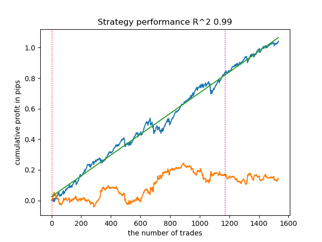
假设我们已经使用自定义测试器训练并选择了一个视觉上令人满意的模型，如下图所示：

现在我们需要在终端中调用导出函数。

导出模型后，3个文件将出现在MetaTrader 5终端的include/mean reversion/文件夹中（在本案例中，使用子目录以避免与其他模型混淆）：

catmodel EURGBP_H1 0.onnx —— 主模型，提供买入和卖出信号
catmodel_m EURGBP_H1 0.onnx —— 附加模型，允许或禁止交易
EURGBP_H1 ONNX include 0.mqh —— 头文件，用于导入这些模型并计算特征。

ONNX模型名称始终以"catmodel"开头，代表CatBoost模型，后接品种名称和时间周期。附加模型以_m后缀标记，代表"基础模型"。头文件名始终以交易品种开头，以模型编号结尾，该编号在导出时指定，以便新导出的模型不会相互覆盖（必要时除外）。

让我们看一下.mqh文件的内容。

#include <Math\Stat\Math.mqh>
#resource "catmodel EURGBP_H1 0.onnx" as uchar ExtModel_EURGBP_H1_0[]
#resource "catmodel_m EURGBP_H1 0.onnx" as uchar ExtModel2_EURGBP_H1_0[]

int PeriodsEURGBP_H1_0[10] = {5,35,65,95,125,155,185,215,245,275};
int Periods_mEURGBP_H1_0[1] = {10};

void fill_araysEURGBP_H1_0( double &features[]) {
   double pr[], ret[];
   ArrayResize(ret, 1);
   for(int i=ArraySize(PeriodsEURGBP_H1_0)-1; i>=0; i--) {
       CopyClose(NULL,PERIOD_H1,1,PeriodsEURGBP_H1_0[i],pr);
       ret[0] = MathMean(pr);
       ArrayInsert(features, ret, ArraySize(features), 0, WHOLE_ARRAY); }
   ArraySetAsSeries(features, true);
}

void fill_arays_mEURGBP_H1_0( double &features[]) {
   double pr[], ret[];
   ArrayResize(ret, 1);
   for(int i=ArraySize(Periods_mEURGBP_H1_0)-1; i>=0; i--) {
       CopyClose(NULL,PERIOD_H1,1,Periods_mEURGBP_H1_0[i],pr);
       ret[0] = MathSkewness(pr);
       ArrayInsert(features, ret, ArraySize(features), 0, WHOLE_ARRAY); }
   ArraySetAsSeries(features, true);
}

首先，连接数学计算库，这是计算均值和偏度所必需的，如果将来需要更改特征计算方式，也可能用于计算分布的其他矩和其他数学运算。接下来，我们将两个ONNX模型作为资源加载，用于生成交易信号。此后，声明用于计算特征的周期数组，这些数组将作为主模型和基础模型的输入数据。

剩余的两个函数用于填充特征值数组。需要提醒您，这些文件是在从Python脚本导出模型时创建的，无需每次都从头编写。只需将其连接到交易EA即可。这样一来，在您希望经过一段时间后重新训练模型时非常方便——只需将其导出到终端，模型就会被更新的版本覆盖，之后重新编译EA而无需对代码进行任何更改。庞大的代码一开始可能令人望而生畏，但实际上，训练过程非常简单：只需运行脚本，再编译EA，整个过程可能只需要几分钟。

现在我们需要创建一个交易EA，该EA将连接此头文件并初始化ONNX模型。

#include <Mean reversion/EURGBP_H1 ONNX include 0.mqh>
#include <Trade\Trade.mqh>
#include <Trade\AccountInfo.mqh>
#property strict
#property copyright "Copyright 2025, Dmitrievsky max."
#property link      "https://www.mql5.com/ru/users/dmitrievsky"
#property version   "1.0"

CTrade mytrade;
CPositionInfo myposition;

input bool Allow_Buy = true;           //Allow BUY
input bool Allow_Sell = true;          //Allow SELL
double main_threshold = 0.5;
double meta_threshold = 0.5;
sinput double   MaximumRisk=0.001;     //Progressive lot coefficient
sinput double   ManualLot=0.01;        //Fixed lot, set 0 if progressive
sinput ulong    OrderMagic = 57633493; //Orders magic
input int max_orders = 3;              //Max positions number
input int orders_time_delay = 5;       //Time delay between positions
input int max_spread = 20;             //Max spread
input int stoploss = 2000;             //Stop loss
input int takeprofit = 200;            //Take profit
input string comment = "mean reversion bot";

static datetime last_time = 0;
#define Ask SymbolInfoDouble(_Symbol, SYMBOL_ASK)
#define Bid SymbolInfoDouble(_Symbol, SYMBOL_BID)


const long  ExtInputShape [] = {1, ArraySize(PeriodsEURGBP_H1_0)};
const long  ExtInputShape2 [] = {1, ArraySize(Periods_mEURGBP_H1_0)};
long     ExtHandle = INVALID_HANDLE, ExtHandle2 = INVALID_HANDLE;

//+------------------------------------------------------------------+
//| Expert initialization function                                   |
//+------------------------------------------------------------------+
int OnInit()
  {
   mytrade.SetExpertMagicNumber(OrderMagic);

   ExtHandle = OnnxCreateFromBuffer(ExtModel_EURGBP_H1_0, ONNX_DEFAULT);
   ExtHandle2 = OnnxCreateFromBuffer(ExtModel2_EURGBP_H1_0, ONNX_DEFAULT);

   if(ExtHandle == INVALID_HANDLE || ExtHandle2 == INVALID_HANDLE)
     {
      Print("OnnxCreateFromBuffer error ", GetLastError());
      return(INIT_FAILED);
     }

   if(!OnnxSetInputShape(ExtHandle, 0, ExtInputShape))
     {
      Print("OnnxSetInputShape 1 failed, error ", GetLastError());
      OnnxRelease(ExtHandle);
      return(-1);
     }

   if(!OnnxSetInputShape(ExtHandle2, 0, ExtInputShape2))
     {
      Print("OnnxSetInputShape 2 failed, error ", GetLastError());
      OnnxRelease(ExtHandle2);
      return(-1);
     }

   const long output_shape[] = {1};
   if(!OnnxSetOutputShape(ExtHandle, 0, output_shape))
     {
      Print("OnnxSetOutputShape 1 error ", GetLastError());
      return(INIT_FAILED);
     }
   if(!OnnxSetOutputShape(ExtHandle2, 0, output_shape))
     {
      Print("OnnxSetOutputShape 2 error ", GetLastError());
      return(INIT_FAILED);
     }

   return(INIT_SUCCEEDED);
  }
//+------------------------------------------------------------------+
//| Expert deinitialization function                                 |
//+------------------------------------------------------------------+
void OnDeinit(const int reason)
  {
//---
   OnnxRelease(ExtHandle);
   OnnxRelease(ExtHandle2);
  }

最重要的是正确初始化每个模型输入数组的维度。其等于头文件中用于特征计算的周期值数组的大小。特征数量与周期值数量相同。

两个模型的输出维度都等于1。

const long  ExtInputShape [] = {1, ArraySize(PeriodsEURGBP_H1_0)};
const long  ExtInputShape2 [] = {1, ArraySize(Periods_mEURGBP_H1_0)};

接下来，我们为模型分配句柄。

ExtHandle = OnnxCreateFromBuffer(ExtModel_EURGBP_H1_0, ONNX_DEFAULT);
ExtHandle2 = OnnxCreateFromBuffer(ExtModel2_EURGBP_H1_0, ONNX_DEFAULT);

我们在EA初始化函数的主体中设置输入和输出的正确维度。

if(!OnnxSetInputShape(ExtHandle, 0, ExtInputShape))
     {
      Print("OnnxSetInputShape 1 failed, error ", GetLastError());
      OnnxRelease(ExtHandle);
      return(-1);
     }

if(!OnnxSetInputShape(ExtHandle2, 0, ExtInputShape2))
     {
      Print("OnnxSetInputShape 2 failed, error ", GetLastError());
      OnnxRelease(ExtHandle2);
      return(-1);
     }

从图表上删除EA后，模型也会被一并删除。

为了加快计算速度，EA在每根新K线开盘时进行交易。现在我们需要看一下如何从模型中获取信号。

void OnTick()
  {
   if(!isNewBar())
      return;

   double features[], features_m[];
   fill_araysEURGBP_H1_0(features);
   fill_arays_mEURGBP_H1_0(features_m);

   double f[ArraySize(PeriodsEURGBP_H1_0)], f_m[ArraySize(Periods_mEURGBP_H1_0)];

   for(int i = 0; i < ArraySize(PeriodsEURGBP_H1_0); i++)
     {
      f[i] = features[i];
     }

   for(int i = 0; i < ArraySize(Periods_mEURGBP_H1_0); i++)
     {
      f_m[i] = features_m[i];
     }

   static vector out(1), out_meta(1);

   struct output
     {
      long           label[];
      float          proba[];
     };

   output out2[], out2_meta[];
   
   OnnxRun(ExtHandle, ONNX_DEBUG_LOGS, f, out, out2);
   OnnxRun(ExtHandle2, ONNX_DEBUG_LOGS, f_m, out_meta, out2_meta);

   double sig = out2[0].proba[1];
   double meta_sig = out2_meta[0].proba[1];

从ONNX模型中接收信号的顺序：

创建features和features_m数组
通过相应的fill_arrays函数，使用特征值填充。
这些数组中元素的顺序与模型应该接收的顺序相反。这就是为什么要创建f和f_m数组，并且要以正确的顺序重写数据。
创建out和out_meta向量，用于告知模型输出向量的维度。
创建output结构体，用于接收预测的0/1标签和概率。概率用于信号计算。
创建输出结构体的out2和out2_meta实例，用于接收信号。
模型启动时需指定输入特征及输出值的维度。它们返回预测结果。
从结构体实例中提取预测值（概率）。

最后，还需探讨如何基于接收到的信号构建开仓逻辑。平仓信号的运作逻辑与开仓信号相反。

// OPEN POSITIONS BY SIGNALS
   if((Ask-Bid < max_spread*_Point) && meta_sig > meta_threshold &&
      AllowTrade(OrderMagic))
      if(countOrders(OrderMagic) < max_orders &&
         CheckMoneyForTrade(_Symbol, LotsOptimized(), ORDER_TYPE_BUY))
        {
         double l = LotsOptimized();
         if(sig < 1-main_threshold && Allow_Buy)
           {
            int res = -1;
            do
              {
               double stop = Bid - stoploss * _Point;
               double take = Ask + takeprofit * _Point;
               res = mytrade.PositionOpen(_Symbol, ORDER_TYPE_BUY, l, Ask, stop, take, comment);
               Sleep(50);
              }
            while(res == -1);
           }
         else
           {
            if(sig > main_threshold && Allow_Sell)
              {
               int res = -1;
               do
                 {
                  double stop = Ask + stoploss * _Point;
                  double take = Bid - takeprofit * _Point;
                  res = mytrade.PositionOpen(_Symbol, ORDER_TYPE_SELL, l, Bid, stop, take, comment);
                  Sleep(50);
                 }
               while(res == -1);
              }
           }
        }

首先，检查第二个模型的信号。如果概率大于0.5，则允许开仓（市场处于必要的模式）。接下来，根据主模型检查条件，该模型预测买入或卖出的可能性。概率小于0.5表示买入，而概率大于0.5则表示卖出。根据条件开仓。

现在我们可以编译EA并在策略测试器中进行测试。

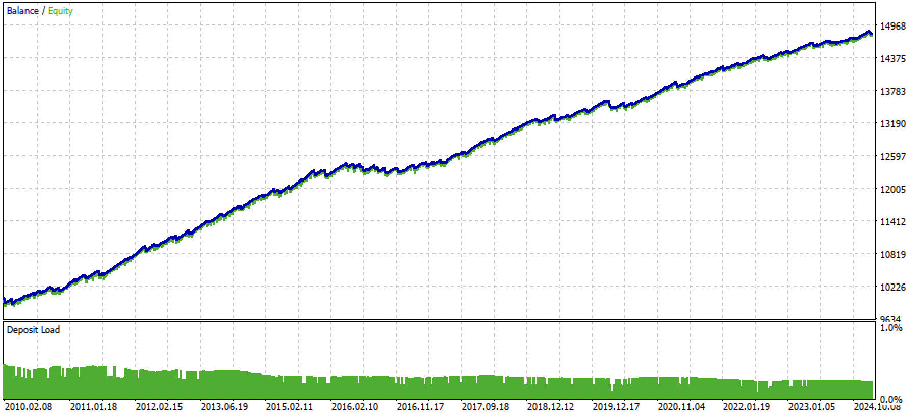
图例3. 使用均值回归策略测试训练后的模型

结论

本文演示了利用机器学习开发均值回归策略的完整流程。文章系统梳理了从交易标注、市场状态识别，到模型训练乃至创建全自动EA的全过程。

文章里包含了全部必要代码，便于读者独立操作。

Python files.zip包含在Python环境中进行开发所需的以下文件：

文件名	描述
mean reversion.py	训练模型的主脚本
labeling_lib.py	带交易标注的模块
tester_lib.py	基于机器学习的自定义策略测试器
export_lib.py	用于将模型以ONNX格式导出至MetaTrader 5终端的库
EURGBP_H1.csv	由MetaTrader 5终端导出的报价文件

MQL5 files.zip包含适用于MetaTrader 5终端的文件：

文件名	描述
mean reversion.ex5	来自本文的编译后的EA
mean reversion.mq5	来自本文的EA源代码
folder Include//Mean reversion	ONNX模型以及用于连接EA的头文件

本文由MetaQuotes Ltd译自俄文
原文地址： https://www.mql5.com/ru/articles/16457

附加的文件 |

下载ZIP

Python_files.zip (1503.93 KB)

MQL5_files.zip (449.31 KB)

注意: MetaQuotes Ltd.将保留所有关于这些材料的权利。全部或部分复制或者转载这些材料将被禁止。

本文由网站的一位用户撰写，反映了他们的个人观点。MetaQuotes Ltd 不对所提供信息的准确性负责，也不对因使用所述解决方案、策略或建议而产生的任何后果负责。

该作者的其他文章

最近评论 | 前往讨论 (91)

Vladimir Levchenko | 3 7月 2025 在 10:48

Maxim Dmitrievsky #:

检查过了，一切正常。附上文章中训练好的模型文件和上面更新的机器人文件。

之后最好重新训练模型，因为文章中附有演示模型。当你理解了 python 脚本后。

您好！
是的，在这个版本中，机器人本身可以正常编译和运行。但模型需要重新训练。
我正在逐渐掌握 python，但还没有完全理解。我在笔记本电脑上滚动了 Rutop 的主版本，并将其更新到当前版本。我安装了所有必要的软件包（pandas、numpa、numpy、catboost、scipy、scikit-learn）。引号已下载。我将报价文件和所有脚本放在 MT5 主目录下的 Files 文件夹中。我在模型训练脚本的代码中写入了路径。
我在 MetaEditore 中更正了脚本代码。我尝试从那里运行脚本。运行过程中出现错误（找不到 python 机器人软件包，试图按照安装其他软件包的方案安装时也出现错误）。通过 python 控制台运行脚本时，也会出现同样的错误。
，您能告诉我该从哪个方向钻研这个主题吗？

[删除] | 3 7月 2025 在 12:07

Vladimir Levchenko #:
您好！
是的，在这个版本中，机器人本身可以正常编译和运行。但模型需要重新训练。
我正在学习 python，但目前还不是一切正常。我在笔记本电脑上运行了 Rutop 的主版本，并将其更新到当前版本。我安装了所有必要的软件包（pandas、numpa、numpy、catboost、scipy、scikit-learn）。引号已下载。我将报价文件和所有脚本放在 MT5 主目录下的 Files 文件夹中。我在模型训练脚本的代码中写入了路径。
我在 MetaEditore 中更正了脚本代码。我尝试从那里运行脚本。运行过程中出现错误（找不到 python 机器人软件包，试图按照安装其他软件包的方案安装时也出现错误）。通过 python 控制台运行脚本时也会出现同样的错误。
你能告诉我应该从哪个方向钻研这个主题吗？

Bots 只是文章中模块所在的根目录（文件夹）。如果脚本在导入模块（附加文件）时没有看到它们，那么请写入文件的完整路径。

或者将所有这些文件扔到与主脚本相同的文件夹中，然后这样做：

Было
from bots.botlibs.labeling_lib import get_labels
from bots.botlibs.tester_lib import test_model
from bots.botlibs.export_lib import export_model_to_ONNX

Стало
from labeling_lib import get_labels
from tester_lib import test_model
from export_lib import export_model_to_ONNX

如果安装 Python 时没有设置 PYTHONPATH，就会出现这种情况。请在互联网上搜索如何为您的系统设置PYTHONPATH。也就是说，Python 看不到光盘上的文件。

或者在互联网上阅读有关导入模块的基础课程。

Vladimir Levchenko | 7 7月 2025 在 15:49

Maxim Dmitrievsky #:

Bots 只是文章中模块所在的根目录（文件夹）。如果脚本在导入模块（附加文件）时没有看到它们，请写入文件的完整路径。

或者将所有这些文件扔到与主脚本相同的文件夹中，然后这样做：

如果安装 Python 时没有设置 PYTHONPATH，就会出现这种情况。请在互联网上搜索如何为您的系统设置PYTHONPATH。也就是说，Python 看不到光盘上的文件。

或者在互联网上阅读有关导入模块的基础课程。

再见，马克西姆。谢谢。几乎所有问题都解决了。最后一个问题。
在训练模型的主脚本中有注释行（154-182）。据我所知，这些是替代交易采样器（标记）。但我无法尝试。如果取消注释任何一个标记（有条件的，第 154-158 行），并注释掉原来的标记（第 149-153 行），脚本将无法启动。
原因何在，应从何处查找？

谢谢 )

[删除] | 7 7月 2025 在 16:41

Vladimir Levchenko #:

日安迈克西姆谢谢几乎所有问题都解决了。最后一个问题。
在训练模型的主脚本中有注释行（154-182）。据我所知，这些是替代交易采样器（标记）。但我无法尝试。如果取消注释任何一个标记（有条件的，第 154-158 行），并且注释了原始标记（第 149-153 行），脚本将无法启动。
原因何在，应从何处查找？

谢谢 )

您好，您需要 Python 解释器写入的日志。

Alexey Klenov | 13 10月 2025 在 14:13

Vladimir Levchenko #:

日安迈克西姆谢谢几乎所有问题都解决了。最后一个问题。
在训练模型的主脚本中有注释行（154-182）。据我所知，这些是替代交易采样器（标记）。但我无法尝试。如果取消注释任何标记（有条件的，第 154-158 行），并且注释了原始标记（第 149-153 行），脚本将无法启动。
原因何在，应从何处查找？

谢谢 )

检查未注释文本是否在同一行上

不应有下划线，如下图所示

交易策略

各种交易策略的分类都是任意的，下面这种分类强调从交易的基本概念上分类。

从新手到专家：使用 MQL5 制作动画新闻标题（一）

在 MetaTrader 5 终端上进行交易时，新闻可访问性是一个关键因素。虽然有很多新闻 API 可用，但许多交易者在访问这些 API 并将其有效集成到他们的交易环境中时仍面临挑战。在本次讨论中，我们的目标是开发一种简化的解决方案，将新闻直接呈现在图表上 —— 也就是最需要新闻的地方。我们将通过构建一个新闻标题 EA 来实现这一目标，该 EA 可以监控并显示来自 API 源的实时新闻更新。

新手在交易中的10个基本错误

新手在交易中会犯的10个基本错误: 在市场刚开始时交易, 获利时不适当地仓促, 在损失的时候追加投资, 从最好的仓位开始平仓, 翻本心理, 最优越的仓位, 用永远买进的规则进行交易, 在第一天就平掉获利的仓位,当发出建一个相反的仓位警示时平仓, 犹豫。

台球优化算法(BOA)

BOA方法灵感源自经典的台球运动，它将寻求最优解的过程模拟为一场游戏：球体致力于落入代表最佳结果的球袋之中。本文将探讨BOA的基本原理、数学模型及其在解决各类优化问题中的效率。