Developing Trend Trading Strategies Using Machine Learning

Introduction

Several types of trading strategies have proven their effectiveness in trading. One such strategy-the mean reversion strategy was covered in a previous article. In this article, I decided to share with the reader some ideas on how machine learning can be used to create trend-based or trend-following strategies.

This article will use a similar approach based on data clustering to identify market regimes. However, the actual trade labelers will differ significantly. Therefore, I recommend first reviewing the first article,and then proceeding to this one as a logical continuation. This will allow you to see the difference between the first and second types of strategies, as well as the differences in labeling training examples. Well then, let's get started!

Approaches to Labeling Data for Trend-Following Strategies

The primary difference between trend-following strategies and mean reversion strategies is that for trend-following strategies, precise identification of the current trend is crucial. For mean reversion strategies, it is sufficient that prices oscillate around a certain average value and frequently cross it. It can be said that these strategies are diametrically opposed. If mean reversion implies a high probability of a reversal in the price movement direction, then trend following implies a continuation of the current trend.

Currency pairs are often categorized as ranging (flat) or trending. Of course, this is a rather conditional classification, as both trends and consolidation zones can be present in either type. Here, the distinction is more based on how frequently they are in one state or the other. In this article, we will not conduct a detailed study of which instruments are truly trending. We will simply test the approach on the EURUSD currency pair, which is considered trending, as opposed to EURGBP, which was examined in the previous article as a ranging pair.

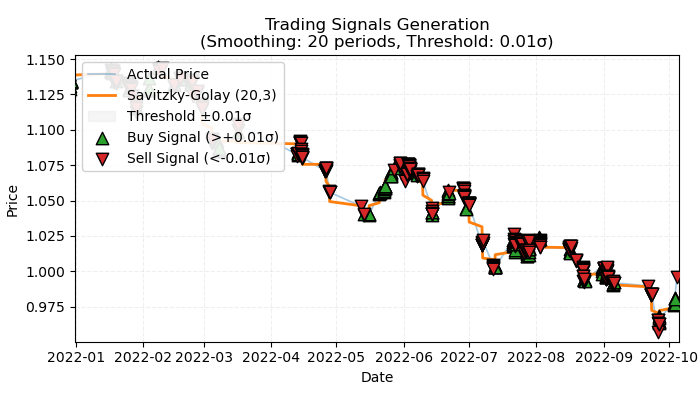
Figure 1. visual representation of labeled trend-based trades

Figure 1 illustrates the fundamental principle that will be used for labeling trend-based trades. To smooth out short-term noise fluctuations, I again used the Savitzky–Golay filter, which was discussed in detail in the previous article. However, instead of calculating price deviations from the filter, as was done last time, we are now interested in the filter's direction as an indicator of the trend. If the direction is positive, a buy trade is labeled; otherwise, a sell trade is labeled. If the direction is undefined, such trades are excluded from the training process. The labeling function incorporates an embedded trend strength filter or threshold, which filters out insignificant trends based on volatility and will be discussed below.

A Basic method for labeling trend-based trades

For a complete understanding of its mechanism, let's explore the trade labeling function from the inside.

@njit
def calculate_labels_trend(normalized_trend, threshold):
    labels = np.empty(len(normalized_trend), dtype=np.float64)
    for i in range(len(normalized_trend)):
        if normalized_trend[i] > threshold:
            labels[i] = 0.0  # Buy (Up trend)
        elif normalized_trend[i] < -threshold:
            labels[i] = 1.0  # Sell (Down trend)
        else:
            labels[i] = 2.0  # No signal
    return labels

def get_labels_trend(dataset, rolling=200, polyorder=3, threshold=0.5, vol_window=50) -> pd.DataFrame:
    smoothed_prices = savgol_filter(dataset['close'].values, window_length=rolling, polyorder=polyorder)
    trend = np.gradient(smoothed_prices)
    vol = dataset['close'].rolling(vol_window).std().values
    normalized_trend = np.where(vol != 0, trend / vol, np.nan)  # Set NaN where vol is 0
    labels = calculate_labels_trend(normalized_trend, threshold)
    dataset = dataset.iloc[:len(labels)].copy()
    dataset['labels'] = labels
    dataset = dataset.dropna()  # Remove rows with NaN
    return dataset

The get_labels_trend function processes the raw data — dataset containing a "close" column (closing prices) and returns a dataframe with an added column of labeled signals.

Key labelling steps:

• Price smoothing. A Savitzky–Golay filter is applied to smooth the closing prices. Parameters include the smoothing window length and polynomial order. The goal is to eliminate noise and highlight the underlying trend.

smoothed_prices = savgol_filter(dataset['close'].values, window_length=rolling, polyorder=polyorder)

• Trend calculation.The gradient of the smoothed prices is computed. The gradient indicates the rate and direction of the price change. A positive gradient signifies an uptrend, a negative one a downtrend. 

trend = np.gradient(smoothed_prices)

• Volatility calculation. Volatility is calculated as the standard deviation of closing prices over a rolling window. This helps assess price variability for normalizing the trend.

vol = dataset['close'].rolling(vol_window).std().values

• Trend normalization. The trend is divided by volatility to account for market variability. 

normalized_trend = np.where(vol != 0, trend / vol, np.nan)

• Label generation. Labels for buy and sell signals are generated based on the normalized trend and a threshold.

labels = calculate_labels_trend(normalized_trend, threshold)

• Threshold application. This value filters out minor gradient deviations. It is selected empirically, typically in the range of 0.01 - 0.5. Trends within the filter boundaries are ignored as insignificant.

We will take this labeling approach as a basis and write additional labelers to have more options for experimentation.

Labeling with strictly profitable trades limitation

The basic approach inherently includes some losing trades, as they can occur at the very end of a trend just before a reversal. This corresponds to real trading system signals, which can be wrong. What matters is the percentage ratio of profitable to losing trades, which should favor profitable ones. However, we can eliminate this flaw by labeling only profitable trades and ignoring losing ones. This helps smooth the equity curve on training and potentially on test data. The code for such labeling is presented below.

@njit
def calculate_labels_trend_with_profit(close, normalized_trend, threshold, markup, min_l, max_l):
    labels = np.empty(len(normalized_trend) - max_l, dtype=np.float64)
    for i in range(len(normalized_trend) - max_l):
        if normalized_trend[i] > threshold:
            # Проверяем условие для Buy
            rand = random.randint(min_l, max_l)
            future_pr = close[i + rand]
            if future_pr >= close[i] + markup:
                labels[i] = 0.0  # Buy (Profit reached)
            else:
                labels[i] = 2.0  # No profit
        elif normalized_trend[i] < -threshold:
            # Проверяем условие для Sell
            rand = random.randint(min_l, max_l)
            future_pr = close[i + rand]
            if future_pr <= close[i] - markup:
                labels[i] = 1.0  # Sell (Profit reached)
            else:
                labels[i] = 2.0  # No profit
        else:
            labels[i] = 2.0  # No signal
    return labels

def get_labels_trend_with_profit(dataset, rolling=200, polyorder=3, threshold=0.5, 
                    vol_window=50, markup=0.00005, min_l=1, max_l=15) -> pd.DataFrame:
    # Smoothing and trend calculation
    smoothed_prices = savgol_filter(dataset['close'].values, window_length=rolling, polyorder=polyorder)
    trend = np.gradient(smoothed_prices)
    
    # Normalizing the trend by volatility
    vol = dataset['close'].rolling(vol_window).std().values
    normalized_trend = np.where(vol != 0, trend / vol, np.nan)
    
    # Removing NaN and synchronizing data
    valid_mask = ~np.isnan(normalized_trend)
    normalized_trend_clean = normalized_trend[valid_mask]
    close_clean = dataset['close'].values[valid_mask]
    dataset_clean = dataset[valid_mask].copy()
    
    # Generating labels
    labels = calculate_labels_trend_with_profit(close_clean, normalized_trend_clean, threshold, markup, min_l, max_l)
    
    # Trimming the dataset and adding labels
    dataset_clean = dataset_clean.iloc[:len(labels)].copy()
    dataset_clean['labels'] = labels
    
    # Filtering the results
    dataset_clean = dataset_clean.dropna()    
    return dataset_clean

Main differences from the basic approach:

• The min_l, parameter has been added, which defines the minimum number of future bars for measuring price change.
• The max_l, parameter has been added, which defines the maximum number of future bars for measuring price change.
• A future bar is selected randomly within the range set by these parameters. Fixed-length checks can be implemented by setting both parameters to the same value.
• If an opened trade at + n bars forward has brought profit, then such a trade is added to the training dataset, otherwise it is labelled as 2.0 (no deal).
• markup parameter has been added, it should be set approximately to the average spread + commission + slippage for the trading instrument, possibly with a margin. This value affects the number of labeled profitable trades — the higher it is, the fewer trades will be labeled as profitable, because they fail to pass this threshold.

Labeling with filter selection option and strictly profitable trades limitation

As in the previous article, we want to have a choice of filters, not just Savitzky–Golay. This allows for more labeling variations and better adaptation of the trading system to different instruments' characteristics. I suggest adding simple moving average, exponential moving average, and spline as additional filters. Just as examples, as you can add your own by analogy.

@njit
def calculate_labels_trend_different_filters(close, normalized_trend, threshold, markup, min_l, max_l):
    labels = np.empty(len(normalized_trend) - max_l, dtype=np.float64)
    for i in range(len(normalized_trend) - max_l):
        if normalized_trend[i] > threshold:
            # Проверяем условие для Buy
            rand = random.randint(min_l, max_l)
            future_pr = close[i + rand]
            if future_pr >= close[i] + markup:
                labels[i] = 0.0  # Buy (Profit reached)
            else:
                labels[i] = 2.0  # No profit
        elif normalized_trend[i] < -threshold:
            # Проверяем условие для Sell
            rand = random.randint(min_l, max_l)
            future_pr = close[i + rand]
            if future_pr <= close[i] - markup:
                labels[i] = 1.0  # Sell (Profit reached)
            else:
                labels[i] = 2.0  # No profit
        else:
            labels[i] = 2.0  # No signal
    return labels

def get_labels_trend_with_profit_different_filters(dataset, method='savgol', rolling=200, polyorder=3, threshold=0.5, 
                    vol_window=50, markup=0.5, min_l=1, max_l=15) -> pd.DataFrame:
    # Smoothing and trend calculation
    close_prices = dataset['close'].values
    if method == 'savgol':
        smoothed_prices = savgol_filter(close_prices, window_length=rolling, polyorder=polyorder)
    elif method == 'spline':
        x = np.arange(len(close_prices))
        spline = UnivariateSpline(x, close_prices, k=polyorder, s=rolling)
        smoothed_prices = spline(x)
    elif method == 'sma':
        smoothed_series = pd.Series(close_prices).rolling(window=rolling).mean()
        smoothed_prices = smoothed_series.values
    elif method == 'ema':
        smoothed_series = pd.Series(close_prices).ewm(span=rolling, adjust=False).mean()
        smoothed_prices = smoothed_series.values
    else:
        raise ValueError(f"Unknown smoothing method: {method}")
    
    trend = np.gradient(smoothed_prices)
    
    # Normalizing the trend by volatility
    vol = dataset['close'].rolling(vol_window).std().values
    normalized_trend = np.where(vol != 0, trend / vol, np.nan)
    
    # Removing NaN and synchronizing data
    valid_mask = ~np.isnan(normalized_trend)
    normalized_trend_clean = normalized_trend[valid_mask]
    close_clean = dataset['close'].values[valid_mask]
    dataset_clean = dataset[valid_mask].copy()
    
    # Generating labels
    labels = calculate_labels_trend_different_filters(close_clean, normalized_trend_clean, threshold, markup, min_l, max_l)
    
    # Trimming the dataset and adding labels
    dataset_clean = dataset_clean.iloc[:len(labels)].copy()
    dataset_clean['labels'] = labels
    
    # Filtering the results
    dataset_clean = dataset_clean.dropna()    
    return dataset_clean

The main change compared to the previous labeling algorithm is the addition of the method parameter, which can take the following values:

• savgol- Savitzky-Golay filter
• spline-spline interpolation
• sma- simple moving average smoothing
• ema- exponential moving average smoothing.

Labeling based on filters with different periods and strictly profitable trades limitation

Let's make our perception of reality complicated and, consequently, the trade labeling method. There is no restriction on using only a single selected smoothing period. Multiple filters of the same type with different periods can be used simultaneously, labeling trades when at least one condition is met. An example of such a sampler is presented below:

@njit
def calculate_labels_trend_multi(close, normalized_trends, threshold, markup, min_l, max_l):
    num_periods = normalized_trends.shape[0]  # Number of periods
    labels = np.empty(len(close) - max_l, dtype=np.float64)
    for i in range(len(close) - max_l):
        # Select a random number of bars forward once for all periods
        rand = np.random.randint(min_l, max_l + 1)
        buy_signals = 0
        sell_signals = 0
        # Check conditions for each period
        for j in range(num_periods):
            if normalized_trends[j, i] > threshold:
                if close[i + rand] >= close[i] + markup:
                    buy_signals += 1
            elif normalized_trends[j, i] < -threshold:
                if close[i + rand] <= close[i] - markup:
                    sell_signals += 1
        # Combine signals
        if buy_signals > 0 and sell_signals == 0:
            labels[i] = 0.0  # Buy
        elif sell_signals > 0 and buy_signals == 0:
            labels[i] = 1.0  # Sell
        else:
            labels[i] = 2.0  # No signal or conflict
    return labels

def get_labels_trend_with_profit_multi(dataset, method='savgol', rolling_periods=[10, 20, 30], polyorder=3, threshold=0.5, 
                                       vol_window=50, markup=0.5, min_l=1, max_l=15) -> pd.DataFrame:
    """
    Generates labels for trading signals (Buy/Sell) based on the normalized trend,
    calculated for multiple smoothing periods.

    Args:
        dataset (pd.DataFrame): DataFrame with data, containing the 'close' column.
        method (str): Smoothing method ('savgol', 'spline', 'sma', 'ema').
        rolling_periods (list): List of smoothing window sizes. Default is [200].
        polyorder (int): Polynomial order for 'savgol' and 'spline' methods.
        threshold (float): Threshold for the normalized trend.
        vol_window (int): Window for volatility calculation.
        markup (float): Minimum profit to confirm the signal.
        min_l (int): Minimum number of bars forward.
        max_l (int): Maximum number of bars forward.

    Returns:
        pd.DataFrame: DataFrame with added 'labels' column:
                      - 0.0: Buy
                      - 1.0: Sell
                      - 2.0: No signal
    """
    close_prices = dataset['close'].values
    normalized_trends = []

    # Calculate normalized trend for each period
    for rolling in rolling_periods:
        if method == 'savgol':
            smoothed_prices = savgol_filter(close_prices, window_length=rolling, polyorder=polyorder)
        elif method == 'spline':
            x = np.arange(len(close_prices))
            spline = UnivariateSpline(x, close_prices, k=polyorder, s=rolling)
            smoothed_prices = spline(x)
        elif method == 'sma':
            smoothed_series = pd.Series(close_prices).rolling(window=rolling).mean()
            smoothed_prices = smoothed_series.values
        elif method == 'ema':
            smoothed_series = pd.Series(close_prices).ewm(span=rolling, adjust=False).mean()
            smoothed_prices = smoothed_series.values
        else:
            raise ValueError(f"Unknown smoothing method: {method}")
        
        trend = np.gradient(smoothed_prices)
        vol = pd.Series(close_prices).rolling(vol_window).std().values
        normalized_trend = np.where(vol != 0, trend / vol, np.nan)
        normalized_trends.append(normalized_trend)

    # Transform list into 2D array
    normalized_trends_array = np.vstack(normalized_trends)

    # Remove rows with NaN
    valid_mask = ~np.isnan(normalized_trends_array).any(axis=0)
    normalized_trends_clean = normalized_trends_array[:, valid_mask]
    close_clean = close_prices[valid_mask]
    dataset_clean = dataset[valid_mask].copy()

    # Generate labels
    labels = calculate_labels_trend_multi(close_clean, normalized_trends_clean, threshold, markup, min_l, max_l)

    # Trim data and add labels
    dataset_clean = dataset_clean.iloc[:len(labels)].copy()
    dataset_clean['labels'] = labels

    # Remove remaining NaN
    dataset_clean = dataset_clean.dropna()
    return dataset_clean

Key points to note (highlighted conceptually):

• The labeling function now accepts a list of arbitrary length containing smoothing period values.
• Filters are calculated for all specified periods in a loop.
• Trend gradients across all filters participate in the labeling function.
• A trade is labeled if at least one buy or sell condition is met, provided there are no opposing signals.

The labeling_lib.py module has been enriched with four new samplers:

def get_labels_trend(dataset, rolling=200, polyorder=3, threshold=0.5, vol_window=50) -> pd.DataFrame:
def get_labels_trend_with_profit(dataset, rolling=200, polyorder=3, threshold=0.5, 
def get_labels_trend_with_profit_different_filters(dataset, method='savgol', rolling=200, polyorder=3, threshold=0.5, 
def get_labels_trend_with_profit_multi(dataset, method='savgol', rolling_periods=[10, 20, 30], polyorder=3, threshold=0.5, 

 Let's stop at these variants. They are quite sufficient for testing the core idea of trend labeling.

Model training and testing process

The core logic for data preparation and training is borrowed from the previous article, so its specifics won't be described in detail. However, there are changes: the entire training cycle is now moved to a separate processing function, providing new capabilities for managing the process.

Previously, trades labeled as 2.0 were simply removed from the training dataset and did not participate in learning. This could lead to information loss due to gaps in the label sequence. But how can this information be incorporated into the trading system if a binary classifier is used and 2.0 labels (no action) represent a 3rd class?

Let's recall that two classifiers are involved in training: the first learns to predict buy/sell labels, and the second learns to predict the current market regime (when to trade and when not to). This means we can migrate examples with 2.0 labels to the second model, thus preserving information instead of discarding it.

def processing(iterations = 1, 
               rolling = [10],
               threshold=0.01,
               polyorder=5,
               vol_window=100,  
               use_meta_dilution = True):
    models = []
    for i in range(iterations):
        data = clustering(dataset, n_clusters=hyper_params['n_clusters'])
        sorted_clusters = data['clusters'].unique()
        sorted_clusters.sort()
        for clust in sorted_clusters:
            clustered_data = data[data['clusters'] == clust].copy()
            if len(clustered_data) < 500:
                print('too few samples: {}'.format(len(clustered_data)))
                continue

            clustered_data = get_labels_trend_with_profit_multi(
                                                    clustered_data,
                                                    method='savgol',
                                                    rolling_periods=rolling,
                                                    polyorder=polyorder,
                                                    threshold=threshold,
                                                    vol_window=vol_window,
                                                    min_l=1,
                                                    max_l=15,   
                                                    markup=hyper_params['markup'])
            
            
            print(f'Iteration: {i}, Cluster: {clust}')
            clustered_data = clustered_data.drop(['close', 'clusters'], axis=1)
            meta_data = data.copy()
            meta_data['clusters'] = meta_data['clusters'].apply(lambda x: 1 if x == clust else 0)
            if use_meta_dilution:
                for dt in clustered_data.index:
                    if clustered_data.loc[dt, 'labels'] == 2.0:
                        if dt in meta_data.index:  # Check if datetime exists in meta_data
                            meta_data.loc[dt, 'clusters'] = 0
            clustered_data = clustered_data.drop(clustered_data[clustered_data.labels == 2.0].index)

            # Синхронизация meta_data с bad_data
            models.append(fit_final_models(clustered_data, meta_data.drop(['close'], axis=1)))
        models.sort(key=lambda x: x[0])
    return models

In the code, it is shown that examples labeled 2.0 in the dataset for the first model are selected in the dataset for the second model by their corresponding dates/rows, and zeros are set in the clusters column. Recalling that ones permit trading, the second model will now predict not only the market regime but also undesirable trade entry points according to the trade sampler. In other words, the second model will now predict both the required market regime and undesirable market entry points.

I suggest using the last sampler immediately, as it incorporates all the best features and has flexible settings.

Let's conduct 10 training cycles with the following settings:

hyper_params = {
    'symbol': 'EURUSD_H1',
    'export_path': '/Users/dmitrievsky/Library/Containers/com.isaacmarovitz.Whisky/Bottles/54CFA88F-36A3-47F7-915A-D09B24E89192/drive_c/Program Files/MetaTrader 5/MQL5/Include/Mean reversion/',
    'model_number': 0,
    'markup': 0.00010,
    'stop_loss':  0.00500,
    'take_profit': 0.00200,
    'periods': [i for i in range(5, 300, 30)],
    'periods_meta': [100],
    'backward': datetime(2000, 1, 1),
    'forward': datetime(2024, 1, 1),
    'full forward': datetime(2026, 1, 1),
    'n_clusters': 10,
    'rolling': [10],
}

The training function itself is called as follows:

dataset = get_features(get_prices())
models = processing(iterations = 10, 
               threshold=0.001,
               polyorder=3,
               vol_window=100,  
               use_meta_dilution = True)

During training, R^2 scores for each pass (cluster) will be displayed:

Iteration: 0, Cluster: 0
R2: 0.9837358133371028
Iteration: 0, Cluster: 1
R2: 0.9002342482016827
Iteration: 0, Cluster: 2
R2: 0.9755114279213657
Iteration: 0, Cluster: 3
R2: 0.9833351908595832
Iteration: 0, Cluster: 4
R2: 0.9537875370012954
Iteration: 0, Cluster: 5
R2: 0.9863566422346429
too few samples: 471
Iteration: 0, Cluster: 7
R2: 0.9852545217737659
Iteration: 0, Cluster: 8
R2: 0.9934196831544163

Let's test the best model from the entire list:

test_model(models[-1][1:],
           hyper_params['stop_loss'], 
           hyper_params['take_profit'], 
           hyper_params['forward'], 
           plt=True)

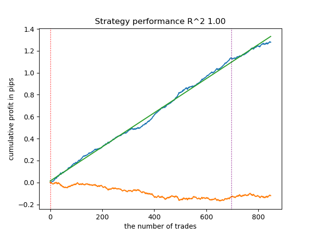
Figure 2. model testing on training and new data

Now we can call the function to export the models to the MetaTrader 5 terminal.

export_model_to_ONNX(model = models[-1],
                     symbol = hyper_params['symbol'],
                     periods = hyper_params['periods'],
                     periods_meta = hyper_params['periods_meta'],
                     model_number = hyper_params['model_number'],
                     export_path = hyper_params['export_path'])

Final model testing and general remarks on the algorithm

My approach is universal, so exporting models to the terminal is done in exactly the same way as described in the previous article.

Let's look at the entire training + test period and the test period separately. The figures show that the equity curve is smoother on the training data than on the test data starting in 2024. Since training was conducted from 2020 to 2024, the test is shown from 2019 to demonstrate that the period before training is also not perfectly smooth.

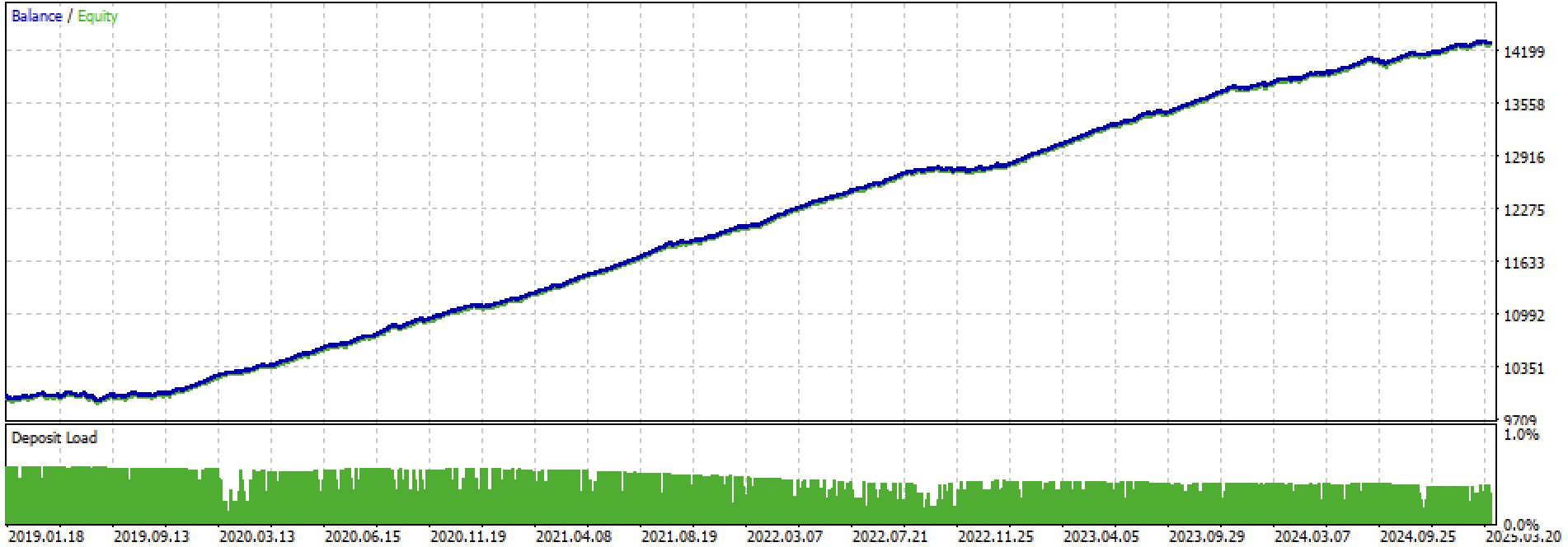
Figure 3. testing from 2019 until 2025.

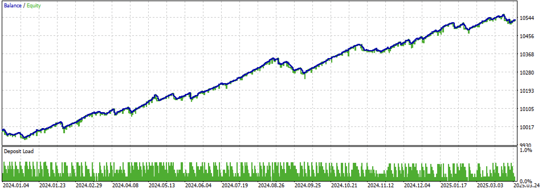
Figure 4. testing on the forward period from early 2024 until 27 March 2025

Based on the conducted experiments, I conclude that trend-following strategies are more finicky in terms of their performance on new data, or this approach does not handle creating such strategies well on the EURUSD pair. Nevertheless, by experimenting with hyperparameter tuning, reasonably good models can be obtained. The drawbacks are partially compensated by the fact that such models can show good results with a very short stop-loss, e.g., in 20 4-digit points. This allows for risk control and timely deactivation of models when they start to fail.

Also, I could not identify any significant set of hyperparameters. I got the impression that the algorithm is fundamentally weak at finding any stable patterns, or such patterns are simply absent.

To combat overfitting, model complexity can be reduced in the fit_final_models() function:

def fit_final_models(clustered, meta) -> list:
    # features for model\meta models. We learn main model only on filtered labels 
    X, X_meta = clustered[clustered.columns[:-1]], meta[meta.columns[:-1]]
    X = X.loc[:, ~X.columns.str.contains('meta_feature')]
    X_meta = X_meta.loc[:, X_meta.columns.str.contains('meta_feature')]
    
    # labels for model\meta models
    y = clustered['labels']
    y_meta = meta['clusters']
    
    y = y.astype('int16')
    y_meta = y_meta.astype('int16')

    # train\test split
    train_X, test_X, train_y, test_y = train_test_split(
        X, y, train_size=0.7, test_size=0.3, shuffle=True)
    
    train_X_m, test_X_m, train_y_m, test_y_m = train_test_split(
        X_meta, y_meta, train_size=0.7, test_size=0.3, shuffle=True)


    # learn main model with train and validation subsets
    model = CatBoostClassifier(iterations=100,
                               custom_loss=['Accuracy'],
                               eval_metric='Accuracy',
                               verbose=False,
                               use_best_model=True,
                               task_type='CPU',
                               thread_count=-1)
    model.fit(train_X, train_y, eval_set=(test_X, test_y),
              early_stopping_rounds=15, plot=False)
    
    # learn meta model with train and validation subsets
    meta_model = CatBoostClassifier(iterations=100,
                                    custom_loss=['F1'],
                                    eval_metric='F1',
                                    verbose=False,
                                    use_best_model=True,
                                    task_type='CPU',
                                    thread_count=-1)
    meta_model.fit(train_X_m, train_y_m, eval_set=(test_X_m, test_y_m),
              early_stopping_rounds=15, plot=False)

    
    R2 = test_model([model, meta_model], hyper_params['stop_loss'], hyper_params['take_profit'], hyper_params['full forward'])
    if math.isnan(R2):
        R2 = -1.0
        print('R2 is fixed to -1.0')
    print('R2: ' + str(R2))

    return [R2, model, meta_model]

The number of iterations controls the number of splits in the model and the number of selected features. Initially, it was 1000 iterations; we reduce it to 100. Early stopping halts training prematurely if the classification error on validation data does not improve for 15 consecutive iterations.

This resulted in a noisier and more uniform, but less "beautiful" equity curve.

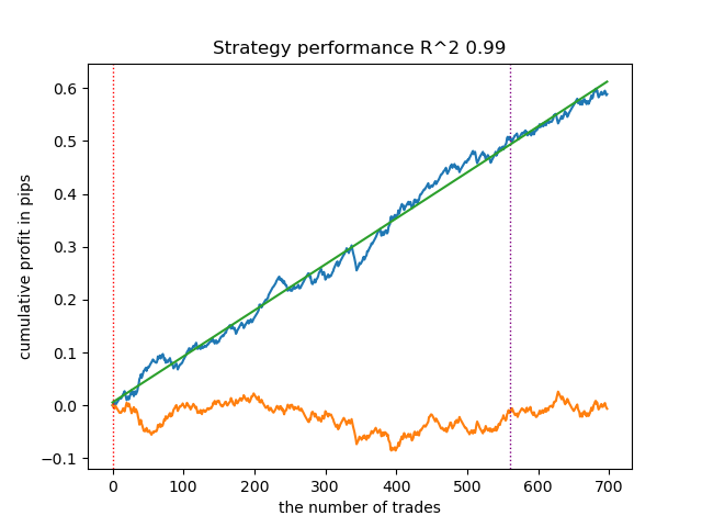
Figure 5. equity curve after reducing model complexity.

Conclusion

Creating trend-following strategies based on clustering and binary classification is more challenging. New insights are needed on how this can be done. A specific problem seems to be financial asset prices moving outside the value range on which the model was trained. Unlike training on ranging instruments, where prices on new data more often correspond to those seen during training. If features based on price differences are applied, the model again demonstrates poor generalization ability.

With this article, I aimed to summarize my experiments with the market regime clustering approach, and ahead of you lie new, even more interesting ideas.

Attached materials:

File name	Description
labeling_lib.py	Updated library of samplers
trend_following.py	Model training script
cat model_EURUSD_H1_0.onnx	Main model, include folder
catmodel_m_EURUSD_H1_0.onnx	Meta-model, include folder
EURUSD_H1_ONNX_include_0.mqh	Header file
trend_following.mq5	Trading Expert Advisor source
trend_following.ex5	Compiled bot