
Data Science and ML (Part 47): Forecasting the Market Using the DeepAR model in Python

Contents
- Introduction
- What is DeepAR?
- Working principles of DeepAR
- Preparing data for the DeepAR model
- Training the DeepAR model in Python
- Real-time market prediction using the DeepAR model
- A multicurrency approach on the DeepAR model
- Conclusion
Introduction
Time series forecasting has never been an easy task in machine learning; several techniques and models have been introduced to tackle this problem, most without definitive success. Linear and non-linear models are often not capable of this task either, despite showing glimpses of decent predictions of time series data.
To tackle time series forecasting, traders have found a resort in neural network-based models such as recurrent neural networks (RNNs).
However, RNNs are more like non-linear models and less like time series models. Those familiar with Auto Regressive Integrated Moving Average (ARIMA) and Vector AutoRegressive (AR) might have noticed this. They do require extra steps to prepare the data into windows to make the neural network aware of time series patterns, despite that they are still not programmed for seasonal patterns that traditional models for time series forecasting acknowledge.

In this article, we are going to discuss the DeepAR model. An autoregressive neural network model. It behaves like both a non-linear model, as it has a neural network, while it has the autoregressive property, which is found in classical time series models like ARIMA.
What is DeepAR?
According to their documentation.
The Amazon SageMaker DeepAR forecasting algorithm is a supervised learning algorithm for forecasting scalar (one-dimensional) time series using recurrent neural networks (RNN). Classical forecasting methods, such as autoregressive integrated moving average (ARIMA) or exponential smoothing (ETS), fit a single model to each individual time series. They then use that model to extrapolate the time series into the future.
In many applications, however, you have many similar time series across a set of cross-sectional units. For example, you might have time series groupings for demand for different products, server loads, and requests for webpages. For this type of application, you can benefit from training a single model jointly over all the time series. DeepAR takes this approach. When your dataset contains hundreds of related time series, DeepAR outperforms the standard ARIMA and ETS methods. You can also use the trained model to generate forecasts for new time series that are similar to the ones it has been trained on.
That being said, let's look at the key principles of this model.
Working Principles of DeepAR
Below are some key-working principles of the DeepAR model.
01: Probabilistic Time-series Forecasting
Deep AR doesn't just produce a single point "point estimate" for future values; it learns the outputs and a full distribution over future points.
This enables the model to express uncertainty and generate prediction intervals or quantiles (e.g., P10, P50, P90). These predictions are valuable for risk-aware decisions.
02: Global Modeling Across Many Series
Unlike traditional forecasting models such as ARIMA and ETS that build separate models for each time series, DeepAR trains a single model jointly on many related time series.
This global model learns shared patterns and improves performance, especially when individual series have limited data. This model can even generalize to new but similar series it hasn't seen before.
03: Autoregressive Recurrent Neural Network Architecture
DeepAR uses a Recurrent Neural Network (RNN) based design (typically with LSTM cells in an autoregressive manner). This means that the model conditions predictions on its own previously predicted values and past observations.
This allows it to capture temporal dependencies such as trends, seasonality, and non-linear dynamics in the data.
04: Use of Static and Dynamic Features
This model is built to handle both dynamic and categorical features.
- Static/categorical features such as product category or region
- Dynamic/time-dependent features such as prices.
This ability sets it apart from non-linear models like XGBoost and vanilla neural networks.
05: Time-Aware Feature Engineering
DeepAR derives time features like day of week, month, etc. from a time series, assisting the model in capturing seasonality and periodic behaviors without extensive manual feature engineering.
This saves us a lot of time crafting those time-based features we usually need in time series forecasting.
The following table lists the derived features for the supported basic time frequencies.
| Frequency of the Time Series | Derived Features |
|---|---|
| Minute | minute-of-hour, hour-of-day, day-of-week, day-of-month, day-of-year. |
| Hour | hour-of-day, day-of-week,day-of-month, day-of-year. |
| Day | day-of-week, day-of-month, day-of-year. |
| Week | day-of-month, week-of-year. |
| Month | month-of-year. |
06: Context and Prediction Window Sampling
This model allows us to control how far in the past and into the future to observe and predict, respectively.
Hyperparameters context_length and prediction_length control how much history and how far ahead the model forecasts respectively.
07: Handling of Missing Values
DeepAR can natively handle missing values in the time series. There is no need for external imputation to help maintain forecast accuracy even with incomplete data.
Preparing data for the DeepAR Model
Now that we understand the core principles of this model, let's implement it in Python and see if the hype is real.
Start by downloading all dependencies found in the file requirements.txt (attached at the end of this article) in your Python virtual environment.
pip install -r requirements.txt
Inside main.py, we start by importing all necessary modules.
import pandas as pd
import torch
import lightning.pytorch as pl
import matplotlib.pyplot as plt
import pytorch_forecasting
from pytorch_forecasting import Baseline, DeepAR, TimeSeriesDataSet, GroupNormalizer
from lightning.pytorch.callbacks import EarlyStopping
from pytorch_forecasting.metrics import SMAPE, MultivariateNormalDistributionLoss, QuantileLoss
from pytorch_forecasting import DeepAR
import MetaTrader5 as mt5
import warnings
Since all machine learning models need data they can learn from, let us import the data from MetaTrader 5.
if not mt5.initialize(): # initialize MetaTrader 5
    print(f"failed to initialize MetaTrader5, Error = {mt5.last_error()}")
    exit()

symbol = "EURUSD"
df = pd.DataFrame(mt5.copy_rates_from_pos(symbol, mt5.TIMEFRAME_H1, 1, 1000))

print(df.head())
Outputs.
         time     open     high      low    close  tick_volume  spread  real_volume
0  1760598000  1.16621  1.16623  1.16559  1.16563         1209       0            0
1  1760601600  1.16561  1.16615  1.16541  1.16602         2113       0            0
2  1760605200  1.16602  1.16680  1.16521  1.16539         3925       0            0
3  1760608800  1.16539  1.16569  1.16431  1.16521         4533       0            0
4  1760612400  1.16518  1.16599  1.16487  1.16591         3948       0            0
We have to format the time from seconds to datetime object(s).
df['time'] = pd.to_datetime(df['time'], unit='s')
We then sort the values according to the time column.
df = df.sort_values("time").reset_index(drop=True)
Outputs.
                 time     open     high      low    close  tick_volume  spread  real_volume
0 2025-10-16 07:00:00  1.16621  1.16623  1.16559  1.16563         1209       0            0
1 2025-10-16 08:00:00  1.16561  1.16615  1.16541  1.16602         2113       0            0
2 2025-10-16 09:00:00  1.16602  1.16680  1.16521  1.16539         3925       0            0
3 2025-10-16 10:00:00  1.16539  1.16569  1.16431  1.16521         4533       0            0
4 2025-10-16 11:00:00  1.16518  1.16599  1.16487  1.16591         3948       0            0
To create a TimeSeriesDataset object (an object useful for preparing a timeseries dataset for pytortch_forecasting models), we need two columns: time_idx and group_id (optional).
df["time_idx"] = (df["time"] - df["time"].min()).dt.total_seconds().astype(int) // 3600
df["symbol"] = symbol
The column time_idx represents the ordering of time for all the rows in the dataframe.
The column symbol is used to group different instruments that are present in the dataframe. In this case, we have one group named EURUSD.
When visualized, the Dataframe looks like this:
                 time     open     high      low    close  tick_volume  spread  real_volume  time_idx  symbol
0 2025-10-16 07:00:00  1.16621  1.16623  1.16559  1.16563         1209       0            0         0  EURUSD
1 2025-10-16 08:00:00  1.16561  1.16615  1.16541  1.16602         2113       0            0         1  EURUSD
2 2025-10-16 09:00:00  1.16602  1.16680  1.16521  1.16539         3925       0            0         2  EURUSD
3 2025-10-16 10:00:00  1.16539  1.16569  1.16431  1.16521         4533       0            0         3  EURUSD
4 2025-10-16 11:00:00  1.16518  1.16599  1.16487  1.16591         3948       0            0         4  EURUSD
Again, the DeepAR model is one-dimensional, meaning that a model is trained on a single variable that it will learn to predict the future self of the variable using its past.
Since we usually look for ways to predict the closing price, the close variable is the only feature we need.
However, the closing price is a continuous variable; trying to predict it might prove challenging even for this model. In time series forecasting, we usually deal with stationary data due to their nature (they have a constant mean and variance over time).
Creating the target variable
For this task, let us train our model to predict the returns;
df["returns"] = (df["close"].shift(-1) - df["close"]) / df["close"]
df = df.dropna().reset_index(drop=True)
We then filter the dataframe into 3 columns required by the timeseries data object.
ts_df = df[["time_idx", "returns", "symbol"]]
When printed, it looks like this.
   time_idx   returns  symbol
0         0  0.000335  EURUSD
1         1 -0.000540  EURUSD
2         2 -0.000154  EURUSD
3         3  0.000601  EURUSD
4         4 -0.000069  EURUSD
With a suitable Dataframe in hand, let us create a TimeSeriesDataset object for training first.
max_encoder_length = 24
max_prediction_length = 6
training_cutoff = df["time_idx"].max() - max_prediction_length

training = TimeSeriesDataSet(
    data=ts_df[ts_df.time_idx <= training_cutoff],
    time_idx="time_idx",
    target="returns",
    group_ids=["symbol"],

    max_encoder_length=max_encoder_length,
    max_prediction_length=max_prediction_length,

    min_encoder_length=1,

    allow_missing_timesteps=True,

    time_varying_known_reals=["time_idx"],
    time_varying_unknown_reals=["returns"],

    target_normalizer=GroupNormalizer(groups=["symbol"],
                                      transformation="log1p")
)
max_encoder_length, tells the model how much to look in the past.
max_prediction_lengh, represents the predictive horizon of the model.
We prepare a similar object for validation data, similar to the one for the training data.
validation = TimeSeriesDataSet.from_dataset(training, ts_df, min_prediction_idx=training_cutoff + 1) As described in the principles, the DeepAR model has a built-in way of creating additional time-based features depending on the given datetime from the dataset.
This is true if, you explicitly use the DeepAR model provided by Amazon SageMaker AI. Unfortunately, I couldn't find good documentation for it, so we will implement the model using the Pytorch Forecasting module with manually added time features.
df["hour"] = df["time"].dt.hour.astype(str)
df["day_of_week"] = df["time"].dt.dayofweek.astype(str)
df["month"] = df["time"].dt.month.astype(str)

ts_df = df[["time_idx", "returns", "symbol", "hour", "day_of_week", "month"]]
Training the DeepAR Model in Python
We need dataloaders for our model (a common practice in PyTorch Forecasting).
batch_size = 64

train_dataloader = training.to_dataloader(train=True, batch_size=batch_size, num_workers=0, batch_sampler="synchronized")
val_dataloader = validation.to_dataloader(train=False, batch_size=batch_size, num_workers=0, batch_sampler="synchronized")
We need a trainer for our model, we will use the lightning module.
# create trainer

trainer = pl.Trainer(
    max_epochs=100,
    accelerator="gpu" if torch.cuda.is_available() else "cpu",
    gradient_clip_val=0.1,
    callbacks=[EarlyStopping(monitor="val_loss", patience=10, mode="min")],
)
We train the model for a maximum of 100 epochs and monitor its validation loss for early stopping (stopping training when the model doesn't improve).
Furthermore, we fit the DeepAR model using the trainer object we just created.
trainer.fit(
    model,
    train_dataloaders=train_dataloader,
    val_dataloaders=val_dataloader,
)
Outputs.
┏━━━┳━━━━━━━━━━━━━━━━━━━━━━━━━━┳━━━━━━━━━━━━━━━━━━━━━━━━━━━━━━━━━━━━━━━━┳━━━━━━━━━┳━━━━━━━┳━━━━━━━━┓
┃   ┃ Name                   ┃ Type                               ┃ Params ┃Mode   ┃FLOPs  ┃
┡━━━╇━━━━━━━━━━━━━━━━━━━━━━━━━━╇━━━━━━━━━━━━━━━━━━━━━━━━━━━━━━━━━━━━━━━━╇━━━━━━━━━╇━━━━━━━╇━━━━━━━━┩
│ 0 │ loss                   │ MultivariateNormalDistributionLoss │      0 │ train │     0 │
│ 1 │ logging_metrics        │ ModuleList                         │      0 │ train │     0 │
│ 2 │ embeddings             │ MultiEmbedding                     │    245 │ train │     0 │
│ 3 │ rnn                    │ LSTM                               │ 22.9 K │ train │     0 │
│ 4 │ distribution_projector │ Linear                             │  1.3 K │ train │     0 │
└───┴────────────────────────┴────────────────────────────────────┴────────┴───────┴───────┘
Trainable params: 24.4 K
Non-trainable params: 0
Total params: 24.4 K
Total estimated model params size (MB): 0
Modules in train mode: 14
Modules in eval mode: 0
Total FLOPs: 0
Epoch 10/99 ━━━━━━━━━━━━━━━━━━━━━━━━━━━━━━━━━━━━━━━━ 933/933 0:00:23 • 0:00:00 40.63it/s v_num: 38.000 train_loss_step: -7.305 val_loss: -60.929 train_loss_epoch: -44.401
After the training process is done, we extract the best model from the trainer.
best_model_path = trainer.checkpoint_callback.best_model_path
best_model = DeepAR.load_from_checkpoint(best_model_path, weights_only=False)
Make predictions for evaluation.
raw_predictions = best_model.predict(val_dataloader, mode="raw", return_x=True)
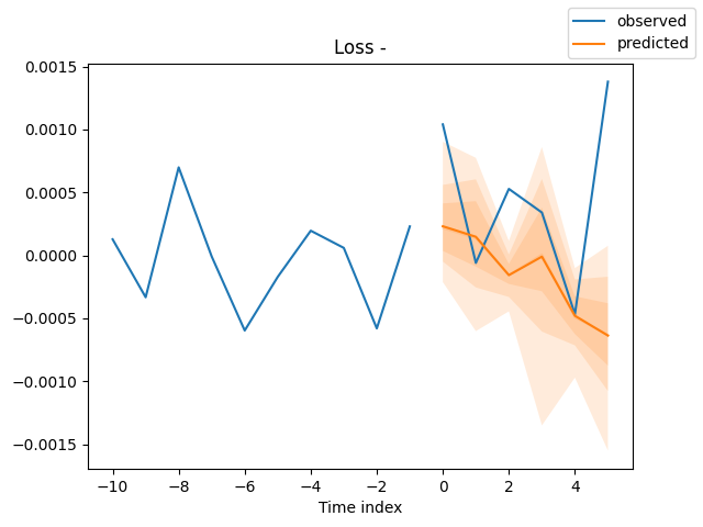
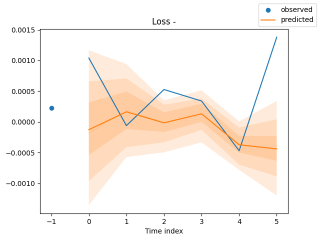
Finally, we plot the predictions for evaluation purposes.
for idx in range(len(raw_predictions.x["decoder_time_idx"])):

    best_model.plot_prediction(
        raw_predictions.x,
        raw_predictions.output,
        idx=idx,
        add_loss_to_title=True
    )

    plt.show()
Outputs (predictions and actual values plotted on the same axis).
Now that we have a way to train the model(s), let us use a model to make useful predictions.
Realtime Market Prediction Using the DeepAR Model
To make our life much easier, we have to split the training process into a separate file, then have a separate function for feature processing and engineering.
Inside the file train.py
import torch
import lightning.pytorch as pl
import matplotlib.pyplot as plt
import pytorch_forecasting
from pytorch_forecasting import DeepAR, TimeSeriesDataSet
from lightning.pytorch.callbacks import EarlyStopping, ModelCheckpoint
from pytorch_forecasting.metrics import MultivariateNormalDistributionLoss
from pytorch_forecasting import DeepAR
# from lightning.pytorch.tuner import Tuner
import os
import config
import warnings

warnings.filterwarnings("ignore")
torch.serialization.add_safe_globals([pytorch_forecasting.data.encoders.GroupNormalizer])
torch.serialization.safe_globals([pytorch_forecasting.data.encoders.GroupNormalizer])

pl.seed_everything(config.random_seed) # set random seed for the lightning module

def run(training: TimeSeriesDataSet,
        train_dataloader: any,
        val_dataloader: any,
        loss: pytorch_forecasting.metrics = MultivariateNormalDistributionLoss(rank=30),
        best_model_name: str=config.best_model_name) -> DeepAR:

    # model's checkpoint

    checkpoint_callback = ModelCheckpoint(
        dirpath=config.models_path,
        filename=best_model_name,
        save_top_k=1,
        mode="min",
        monitor="val_loss"
    )

    # create trainer

    trainer = pl.Trainer(
        max_epochs=config.num_epochs,
        accelerator="gpu" if torch.cuda.is_available() else "cpu",
        gradient_clip_val=config.grad_clip,
        callbacks=[EarlyStopping(monitor="val_loss", patience=config.patience, mode="min"), checkpoint_callback],
        logger=False,
    )

    # create DeepAR model

    model = DeepAR.from_dataset(
        training,
        learning_rate=config.learning_rate,
        hidden_size=config.hidden_size,
        rnn_layers=config.rnn_layers,
        dropout=config.dropout,

        # --- probabilistic forecasting ---
        loss=loss,

        log_interval=config.log_interval,
        log_val_interval=config.log_val_interval,
    )

    res = None
    try:
        # find the optimal learning rate

        """
        res = Tuner(trainer).lr_find(
            model, train_dataloaders=train_dataloader, val_dataloaders=val_dataloader, early_stop_threshold=1000.0, max_lr=0.3,
        )

        # and plot the result - always visually confirm that the suggested learning rate makes sense
        print(f"suggested learning rate: {res.suggestion()}")
        fig = res.plot(show=True, suggest=True)
        fig.savefig(os.path.join(config.images_path, "lr_finder.png"))
        """

        # fit the model

        trainer.fit(
            model,
            train_dataloaders=train_dataloader,
            val_dataloaders=val_dataloader,
        )

    except Exception as e:
        raise RuntimeError(e)

    best_model_path = checkpoint_callback.best_model_path
    best_model = DeepAR.load_from_checkpoint(best_model_path, weights_only=False)

    # make probabilistic forecasts

    raw_predictions = best_model.predict(val_dataloader, mode="raw", return_x=True)

    # plot predictions

    # for idx in range(config.max_prediction_length):
    for idx in range(len(raw_predictions.x["decoder_time_idx"])):
        best_model.plot_prediction(
            raw_predictions.x,
            raw_predictions.output,
            idx=idx,
            add_loss_to_title=True
        )

        plt.savefig(os.path.join(config.images_path, "deepar_forecast_{}.png".format(idx+1)))
        # plt.show()

    return model
Since training a model is a resource-intensive process and certainly not the right thing to do frequently. We need a function for loading a pre-trained (saved) model.
Inside main.py
def load_model():
    global model

    try:
        model = DeepAR.load_from_checkpoint(
            checkpoint_path=os.path.join(config.models_path, config.best_model_name+".ckpt"),
            weights_only=False,
        )
    except Exception as e:
        print(f"Failed to load model from checkpoint: {e}")
        model = None
        return False

    return True
Since we need to deploy the same feature collection and engineering to the data before passing it to the inference model. It is wise to wrap all the required processes in a standalone function.
def feature_engineering(df: pd.DataFrame) -> pd.DataFrame:

    # convert time in seconds to datetime
    df['time'] = pd.to_datetime(df['time'], unit='s')
    df = df.sort_values("time").reset_index(drop=True)

    # print(df.head())

    df["time_idx"] = np.arange(len(df))
    df["symbol"] = symbol

    # print(df.head())

    # instead of using close price, which is very hard to predict, let's use close price returns

    df["returns"] = (df["close"].shift(-1) - df["close"]) / df["close"]
    df = df.dropna().reset_index(drop=True)

    df["hour"] = df["time"].dt.hour.astype(str)
    df["day_of_week"] = df["time"].dt.dayofweek.astype(str)
    df["month"] = df["time"].dt.month.astype(str)

    return df[["time_idx", "returns", "symbol", "hour", "day_of_week", "month"]]
Inside a function training_job,which will be placed on a schedule. For a scheduled training, we start by collecting the data and feature engineering.
Inside the file main.py
def training_job():
    global model

    # ----- feature engineering -----

    try:
        df = pd.DataFrame(mt5.copy_rates_from_pos(symbol, timeframe, config.train_start_bar, config.train_total_bars))
        ts_df = feature_engineering(df)
    except Exception as e:
        print(f"Failed to get historical data from MetaTrader 5: {e}")
        return

    print(ts_df.head())
After getting the raw data in a pandas.DataFrame we need to create TimeSeriesData objects and loaders similarly to how we did previously.
def training_job():
    global model

    # ----- feature engineering -----

    try:
        df = pd.DataFrame(mt5.copy_rates_from_pos(symbol, timeframe, config.train_start_bar, config.train_total_bars))
        ts_df = feature_engineering(df)
    except Exception as e:
        print(f"Failed to get historical data from MetaTrader 5: {e}")
        return

    print(ts_df.head())

    # ----- create timeseries datasets and dataloaders -----

    training_cutoff = ts_df["time_idx"].max() - config.max_prediction_length

    training = TimeSeriesDataSet(
        data=ts_df[ts_df.time_idx <= training_cutoff],
        time_idx="time_idx",
        target="returns",
        group_ids=["symbol"],

        max_encoder_length=config.max_encoder_length,
        max_prediction_length=config.max_prediction_length,

        min_encoder_length=config.min_encoder_length,
        # min_prediction_length=1,

        allow_missing_timesteps=True,

        time_varying_known_categoricals=["hour", "day_of_week", "month"],

        time_varying_known_reals=["time_idx"],
        time_varying_unknown_reals=["returns"],

        target_normalizer=GroupNormalizer(groups=["symbol"],
                                        transformation="log1p")
    )

    validation = TimeSeriesDataSet.from_dataset(training, ts_df, min_prediction_idx=training_cutoff + 1)

    train_dataloader = training.to_dataloader(train=True, batch_size=config.batch_size, num_workers=config.num_workers, batch_sampler="synchronized")
    val_dataloader = validation.to_dataloader(train=False, batch_size=config.batch_size, num_workers=config.num_workers, batch_sampler="synchronized")

    model = train.run(training=training,
              train_dataloader=train_dataloader,
              val_dataloader=val_dataloader,
              loss=MultivariateNormalDistributionLoss(rank=30),
              best_model_name=config.best_model_name)
Finally, we schedule the training operation after some specified time interval in minutes using the Schedule module.
import schedule

#....
#....

schedule.every(config.train_interval_minutes).minutes.do(training_job)
Notice that most variables have the pattern (config.some_variable). This is because most variables are stored within a file named config.py
With all the training procedures in place, we need a final function for receiving the latest ticks and rates from MetaTrader 5 and using that information in executing final trading decisions.
def trading_loop():

    global model
    if model is None:
        if not load_model():
            print("Model not loaded, skipping trading loop.")
            return False
The first thing is to ensure that a global variable named model has an object in place, if not, we load a best model for that particular instrument and timeframe.
Upon a successful model reading, we get real-time data and do the feature engineering processes similarly to how we did during training.
    try:
        df = pd.DataFrame(mt5.copy_rates_from_pos(symbol, timeframe, 1, config.max_encoder_length + config.max_prediction_length))
        ts_df = feature_engineering(df)
    except Exception as e:
        print(f"Failed to get realtime data from MetaTrader 5: {e}")
        return False
We then pass the data to a model object, and obtain the predictions.
Since we have a single group in the training data, we flatten the 2-dimensional array to a 1-dimensional NumPy array.
    predictions = model.predict(data=ts_df, mode="prediction")
    predictions = np.array(predictions).ravel()
Since we trained the model to predict 6 steps using the variable max_prediction_length, the model will always return 6 predicted values for 6 consecutive bars beyond the last known observation.
We have to choose which bar we want to use the prediction for, whatever it is we want (in this case, for setting our stop loss and take profit values).
    forecast_index = -1  # last-step forecast

    predicted_return = predictions[forecast_index]
We have to be mindful of how we crafted the target variable during training because that tells us how we should treat and use the predicted values.
In this case, we trained the model to predict the daily fractional returns. To get an estimated value on the market, we have to multiply the value by the latest closing price (remember the returns were calculated on the closing prices).
price_delta = predicted_return * df["close"].iloc[-1]
We will use this price value from the market to craft our trade's stop loss(es) and take profit(s) while also using the predicted return magnitude as our trading signal (i.e, if the predicted return is negative, that is a bearish signal, and the opposite for a bullish signal).
    # ------------ sl and tp according to model predictions ------------

    if predicted_return > 0:

        tp = round(ask + price_delta, digits)
        sl = round(ask - abs(price_delta), digits)

        if not is_valid_sl_tp(sl=sl, tp=tp, price=ask):
            return

        if not pos_exists(magic_number=m_trade.magic_number, symbol=symbol, pos_type=mt5.POSITION_TYPE_BUY):
            if not m_trade.buy(symbol=symbol, volume=min_lotsize, price=ask, sl=sl, tp=tp):
                print(f"Buy order failed, Error = {mt5.last_error()} | price= {ask}, sl= {sl}, tp= {tp}")

    else:

        tp = round(bid - abs(price_delta), digits)
        sl = round(bid + abs(price_delta), digits)

        if not is_valid_sl_tp(sl=sl, tp=tp, price=bid):
            return

        if not pos_exists(magic_number=m_trade.magic_number, symbol=symbol, pos_type=mt5.POSITION_TYPE_SELL):
            if not m_trade.sell(symbol=symbol, volume=min_lotsize, price=bid, sl=sl, tp=tp):
                print(f"Sell order failed, Error = {mt5.last_error()} | price= {bid}, sl= {sl}, tp= {tp}")
Notice something familiar?
The modules: m_trade, m_symbol, and others are MQL5-like modules made to make our life easier in Python as in MQL5.
Below is how they were declared inside main.py.
import MetaTrader5 as mt5
from Trade.PositionInfo import CPositionInfo
from Trade.SymbolInfo import CSymbolInfo
from Trade.Trade import CTrade

# --------------- configure metatrader5 modules -------------------

if not mt5.initialize(): # initialize MetaTrader 5
    print(f"failed to initialize MetaTrader5, Error = {mt5.last_error()}")
    exit()

m_position = CPositionInfo(mt5_instance=mt5)
m_trade = CTrade(mt5_instance=mt5, magic_number=123456, filling_type_symbol=symbol, deviation_points=100)
m_symbol = CSymbolInfo(mt5_instance=mt5)

m_symbol.name(symbol_name=symbol) # set symbol name
That being said, when the file main.py is run, our simple bot was able to trigger its very first trading operation.
A MultiCurrency Approach On the DeepAR Model
As discussed on the core principles of the DeepAR model, that it is capable of modelling across different time series. Some say it's even better when this model is given different series that exhibit similar patterns, as the learned patterns are reshared, making the model generalize better.
To make it multicurrency we have to feed our model with data from all the instruments we want.
We will follow the same approach with different tweaks in data collection and handling 2-dimensional predictions provided by the model for different time series and windows (predictive horizons).
Instead of having a single variable for a specified symbol, we now have a multi-symbol array.
symbols = [
    "EURUSD",
    "GBPUSD",
    "USDJPY",
    "USDCHF",
    "AUDUSD",
    "USDCAD",
    "NZDUSD"
]

timeframe = mt5.TIMEFRAME_D1
This time we collect data (rates) from MetaTrader 5 across various symbols.
We append all new rows at the end of a big dataframe named ts_df.
def training_job():
    global model

    # -------- feature engineering ---------

    ts_df = pd.DataFrame()
    for symbol in symbols:
        try:

            df = pd.DataFrame(mt5.copy_rates_from_pos(symbol, timeframe, config.train_start_bar, config.train_total_bars))
            temp_df = feature_engineering(df, symbol)

            ts_df = pd.concat([ts_df, temp_df], axis=0, ignore_index=True)

        except Exception as e:
            print(f"Failed to get historical data from MetaTrader 5: {e} for symbol {symbol}")
            continue

    print(ts_df.head())
    print(ts_df.tail())
Outputs.
   time_idx   returns  symbol hour day_of_week month
0         0  0.023229  EURUSD    0           2     4
1         1  0.013703  EURUSD    0           3     4
2         2 -0.000493  EURUSD    0           4     4
3         3 -0.006018  EURUSD    0           0     4
4         4  0.010389  EURUSD    0           1     4
      time_idx   returns  symbol hour day_of_week month
1248       174  0.006002  NZDUSD    0           1    12
1249       175 -0.001272  NZDUSD    0           2    12
1250       176 -0.001670  NZDUSD    0           3    12
1251       177 -0.002759  NZDUSD    0           4    12
1252       178  0.000017  NZDUSD    0           0    12
Inside the function trading_loop, we collect data similarly to how we did during training (this time within a for loop).
    # ----------- get realtime data from MetaTrader 5 -----------

    ts_df = pd.DataFrame()
    for symbol in symbols:
        try:

            df = pd.DataFrame(mt5.copy_rates_from_pos(symbol, timeframe, 1, config.max_encoder_length + config.max_prediction_length))
            temp_df = feature_engineering(df, symbol)

            ts_df = pd.concat([ts_df, temp_df], axis=0, ignore_index=True)

        except Exception as e:

            print(f"Failed to get realtime data from MetaTrader 5: {e} for symbol {symbol}")
            continue
We need another loop for multiple symbols (multicurrency).
    # ---------- use the model to make predictions ----------

    predictions = model.predict(data=ts_df, mode="prediction")
    predictions = np.array(predictions)
    # print("Predictions: ", predictions)

    forecast_index = -1  # last-step forecast

    for idx, (symbol, m_trade, m_symbol) in enumerate(zip(symbols, m_trades, m_symbols)):

        # get latest symbol info

        if not m_symbol.refresh_rates():
            print(f"failed to refresh rates for symbol {symbol}, Error = {mt5.last_error()}")
            return

        min_lotsize = m_symbol.lots_min()

        ask = m_symbol.ask()
        bid = m_symbol.bid()

        # ------------ Get a corresponding prediction -----------

        predicted_return = predictions[idx][forecast_index]
        price_delta = predicted_return * df["close"].iloc[-1]

        digits = m_symbol.digits()

        # ------------ sl and tp according to model predictions ------------

        if predicted_return > 0:

            tp = round(ask + price_delta, digits)
            sl = round(ask - abs(price_delta), digits)

            if not is_valid_sl_tp(sl=sl, tp=tp, price=ask, m_symbol=m_symbol):
                return

            if not pos_exists(magic_number=m_trade.magic_number, symbol=symbol, pos_type=mt5.POSITION_TYPE_BUY, m_symbol=m_symbol):
                if not m_trade.buy(symbol=symbol, volume=min_lotsize, price=ask, sl=sl, tp=tp):
                    print(f"Buy order failed, Error = {mt5.last_error()} | price= {ask}, sl= {sl}, tp= {tp}")

        else:

            tp = round(bid - abs(price_delta), digits)
            sl = round(bid + abs(price_delta), digits)

            if not is_valid_sl_tp(sl=sl, tp=tp, price=bid, m_symbol=m_symbol):
                return

            if not pos_exists(magic_number=m_trade.magic_number, symbol=symbol, pos_type=mt5.POSITION_TYPE_SELL, m_symbol=m_symbol):
                if not m_trade.sell(symbol=symbol, volume=min_lotsize, price=bid, sl=sl, tp=tp):
                    print(f"Sell order failed, Error = {mt5.last_error()} | price= {bid}, sl= {sl}, tp= {tp}")
With multi-groups assigned to our model during training, the inference model will produce a 2-dimensional array of predictions with the shape of (group_ids, predictions).
        predicted_return = predictions[idx][forecast_index]
        price_delta = predicted_return * df["close"].iloc[-1]
Since this bot is now a multicurrency one, we have to handle the classes SymbolInfo and CTrade differently for each instrument.
m_trades = [CTrade(mt5_instance=mt5, magic_number=123456, filling_type_symbol=symbol, deviation_points=100) for symbol in symbols]

m_symbols = []
for symbol in symbols:
    s = CSymbolInfo(mt5_instance=mt5)
    s.name(symbol)
    m_symbols.append(s)
After training the model, we should be able to receive trades from all specified instruments.
The Bottom Line
The DeepAR model is a solid choice for probabilistic time-series forecasting, but it has some drawbacks that must be acknowledged, including its assumption that future values depend mostly on the past (something which isn't always true).
Just like classical models for time series forecasting, it depends on data stationarity, assuming that similar dynamics in the data repeat over time. As we all know, financial markets change rapidly, and there is no such thing as stationarity most of the time.
For now, there is no way of testing the effectiveness of this particular model in an actual trading environment; we can only rely on the predicted plots for testing how close the model's forecasts are to the true values from the market.
Peace out.
Attachments Table
| Filename | Description & Usage |
|---|---|
| main.py | The main Python file for assembling all modules, Machine learning models training, and opening trades in MetaTrader 5. |
| configs.py | A configuration Python file, it has all the necessary variables. It gives our project a global space for tuning. |
| train.py | Contains a function and modules for training the DeepAR model. |
| error_description.py | It has functions for interpreting MetaTrader 5 error codes into human-readable messages (errors). |
| Trade/ | A similar directory to MQL5/Include/Trade. This path has Python modules similar to the standard trade class libraries. |
| requirements.txt | Contains all Python dependencies and their version(s), used in this project. |
Warning: All rights to these materials are reserved by MetaQuotes Ltd. Copying or reprinting of these materials in whole or in part is prohibited.
This article was written by a user of the site and reflects their personal views. MetaQuotes Ltd is not responsible for the accuracy of the information presented, nor for any consequences resulting from the use of the solutions, strategies or recommendations described.

- Free trading apps
- Over 8,000 signals for copying
- Economic news for exploring financial markets
You agree to website policy and terms of use
Very interesting article!
Do you have any books I can check to get deeper on this topics?
I have read about ARIMAS, GARCH and VAR, but don't know where to look more into this ARIMAs and ML models!