Algorithmic Trading Strategies: AI and Its Road to Golden Pinnacles

Introduction

The evolution of understanding the capabilities of machine learning methods in trading has resulted in the creation of different algorithms. They are equally good at the same task, but fundamentally different. This article will consider a unidirectional trending trading system again in the case of gold, but using a clustering algorithm.

• The previous article described two causal inference algorithms for creating a similar trending strategy for gold.
• The article on time series clustering discussed different ways of clustering in trading tasks.
• The creation of a mean-reversion strategy using a clustering algorithm was presented to the public earlier.
• The development of a clustering-based trend trading system has also highlighted capabilities of this approach.

Considering this important approach to the analysis and forecasting of time series from different angles, it is possible to determine its advantages and disadvantages in comparison with other ways of creating trading systems which are based solely on the analysis and forecasting of financial time series. In some cases, these algorithms become quite effective and surpass classical approaches both in terms of the speed of creation and the quality of the resulting trading systems.

In this article, we will focus on unidirectional trading, where the algorithm will only open buy or sell trades. CatBoost and K-Means algorithms will be used as basic algorithms. CatBoost is a basic model that performs functions of a binary classifier for classifying trades. Whereas, K-Means is used to determine market modes at the preprocessing phase.

Preparing for work and importing modules

import math
import pandas as pd
from datetime import datetime
from catboost import CatBoostClassifier

from sklearn.model_selection import train_test_split
from sklearn.cluster import KMeans

from bots.botlibs.labeling_lib import *
from bots.botlibs.tester_lib import tester_one_direction
from bots.botlibs.export_lib import export_model_to_ONNX

import time

The code uses only reliable and verified publicly available packages such as:

• Pandas — responsible for working with data tables (dataframes)
• Scikit-learn — contains various functions for preprocessing and machine learning, including clustering algorithms.
• CatBoost — a powerful gradient boosting algorithm from Yandex

The individual modules I created have been imported:

• labeling_lib — contains sampler functions for marking up trades
• tester_lib — contains testers of machine learning-based strategies.
• export_lib — a module for exporting trained models to Meta Trader 5 in ONNX format

Getting data and creating features

def get_prices() -> pd.DataFrame:
    p = pd.read_csv('files/'+hyper_params['symbol']+'.csv', sep='\s+')
    pFixed = pd.DataFrame(columns=['time', 'close'])
    pFixed['time'] = p['<DATE>'] + ' ' + p['<TIME>']
    pFixed['time'] = pd.to_datetime(pFixed['time'], format='mixed')
    pFixed['close'] = p['<CLOSE>']
    pFixed.set_index('time', inplace=True)
    pFixed.index = pd.to_datetime(pFixed.index, unit='s')
    return pFixed.dropna()

The code implements the download of quotes from a file, for the convenience of obtaining data from various sources. Only closing prices are used. Based on this data, features are created.

def get_features(data: pd.DataFrame) -> pd.DataFrame:
    pFixed = data.copy()
    pFixedC = data.copy()
    count = 0

    for i in hyper_params['periods']:
        pFixed[str(count)] = pFixedC.rolling(i).std()
        count += 1
    
    for i in hyper_params['periods_meta']:
        pFixed[str(count)+'meta_feature'] = pFixedC.rolling(i).std()
        count += 1

Features are divided into two groups:

1. The main features for training a basic model that predicts the direction of trading.
2. Additional meta-features for clustering. They are used to divide the source data into clusters (market modes).

In this example, volatility (standard deviations of prices in sliding windows of a given period) is used as features. But we will also test other features, such as moving averages and skewness of distributions.

Clustering of market modes

def clustering(dataset, n_clusters: int) -> pd.DataFrame:
    data = dataset[(dataset.index < hyper_params['forward']) & (dataset.index > hyper_params['backward'])].copy()
    meta_X = data.loc[:, data.columns.str.contains('meta_feature')]
    data['clusters'] = KMeans(n_clusters=n_clusters).fit(meta_X).labels_
    return data

The function gets a dataframe with prices and features and uses additional meta-features to cluster into a given number of clusters (usually, 10). The K-Means algorithm is used for clustering. After that, each row of the dataframe is assigned a cluster label that corresponds to this observation. And the dataframe is returned with an additional "clusters" column.

A function for training classifiers

def fit_final_models(clustered, meta) -> list:
    # features for model\meta models. We learn main model only on filtered labels 
    X, X_meta = clustered[clustered.columns[:-1]], meta[meta.columns[:-1]]
    X = X.loc[:, ~X.columns.str.contains('meta_feature')]
    X_meta = X_meta.loc[:, X_meta.columns.str.contains('meta_feature')]
    
    # labels for model\meta models
    y = clustered['labels']
    y_meta = meta['clusters']
    
    y = y.astype('int16')
    y_meta = y_meta.astype('int16')

    # train\test split
    train_X, test_X, train_y, test_y = train_test_split(
        X, y, train_size=0.7, test_size=0.3, shuffle=True)
    
    train_X_m, test_X_m, train_y_m, test_y_m = train_test_split(
        X_meta, y_meta, train_size=0.7, test_size=0.3, shuffle=True)


    # learn main model with train and validation subsets
    model = CatBoostClassifier(iterations=500,
                               custom_loss=['Accuracy'],
                               eval_metric='Accuracy',
                               verbose=False,
                               use_best_model=True,
                               task_type='CPU',
                               thread_count=-1)
    model.fit(train_X, train_y, eval_set=(test_X, test_y),
              early_stopping_rounds=25, plot=False)
    
    # learn meta model with train and validation subsets
    meta_model = CatBoostClassifier(iterations=300,
                                    custom_loss=['F1'],
                                    eval_metric='F1',
                                    verbose=False,
                                    use_best_model=True,
                                    task_type='CPU',
                                    thread_count=-1)
    meta_model.fit(train_X_m, train_y_m, eval_set=(test_X_m, test_y_m),
              early_stopping_rounds=15, plot=False)

    
    R2 = test_model_one_direction([model, meta_model],
                                hyper_params['stop_loss'], 
                                hyper_params['take_profit'],
                                hyper_params['full forward'],
                                hyper_params['backward'],
                                hyper_params['markup'],
                                hyper_params['direction'],
                                plt=False)
    if math.isnan(R2):
        R2 = -1.0
        print('R2 is fixed to -1.0')
    print('R2: ' + str(R2))

    return [R2, model, meta_model]

Two models are used for training. The first is trained on basic features and labels, and the second one is trained on meta-features and meta-labels. If for the first model trade directions are the labels, for the second model cluster numbers are the labels. 1 — if the data corresponds to the required cluster, and 0 — if the data corresponds to all other clusters. 

Before training, the data is divided into training and validation data in a 70/30 ratio, so that the CatBoost algorithm is less overfitted. It uses validation data to stop early, when the error stops falling on them during the learning process. Then the best model is selected, which has the smallest prediction error on the validation data.

After training the models, they are passed to the testing function to estimate the balance curve using R^2. This is necessary for the subsequent sorting of models and selecting the best one.

Model testing function

def test_model_one_direction( 
               result: list, 
               stop: float, 
               take: float, 
               forward: float, 
               backward: float, 
               markup: float,
               direction: str, 
               plt = False):
    
    pr_tst = get_features(get_prices())
    X = pr_tst[pr_tst.columns[1:]]
    X_meta = X.copy()
    X = X.loc[:, ~X.columns.str.contains('meta_feature')]
    X_meta = X_meta.loc[:, X_meta.columns.str.contains('meta_feature')]

    pr_tst['labels'] = result[0].predict_proba(X)[:,1]
    pr_tst['meta_labels'] = result[1].predict_proba(X_meta)[:,1]
    pr_tst['labels'] = pr_tst['labels'].apply(lambda x: 0.0 if x < 0.5 else 1.0)
    pr_tst['meta_labels'] = pr_tst['meta_labels'].apply(lambda x: 0.0 if x < 0.5 else 1.0)
    return tester_one_direction(pr_tst, stop, take, forward, backward, markup, direction, plt)

The function accepts two trained models (the main and the meta-model), as well as the remaining parameters necessary for testing in a custom strategy tester. Then, a dataframe with prices and features is created again, which are transmitted to these models for predictions. The received predictions are recorded in the "labels" and "meta_labels" columns of this dataframe.

At the very end, the custom tester function is called, which is located in the plug-in module tester_lib.py. It performs model testing on history and returns an estimate of R^2.

Trade markup function

The labeling_lib.py module contains a sampler designed to mark trades only in the selected direction:

@njit
def calculate_labels_one_direction(close_data, markup, min, max, direction):
    labels = []
    for i in range(len(close_data) - max):
        rand = random.randint(min, max)
        curr_pr = close_data[i]
        future_pr = close_data[i + rand]

        if direction == "sell":
            if (future_pr + markup) < curr_pr:
                labels.append(1.0)
            else:
                labels.append(0.0)
        if direction == "buy":
            if (future_pr - markup) > curr_pr:
                labels.append(1.0)
            else:
                labels.append(0.0)
    return labels

def get_labels_one_direction(dataset, markup, min = 1, max = 15, direction = 'buy') -> pd.DataFrame:
    close_data = dataset['close'].values
    labels = calculate_labels_one_direction(close_data, markup, min, max, direction)
    dataset = dataset.iloc[:len(labels)].copy()
    dataset['labels'] = labels
    dataset = dataset.dropna()
    return dataset

The main learning loop

# LEARNING LOOP
dataset = get_features(get_prices()) 	// getting prices and features
models = [] 				// making empty list of models

for i in range(1):							// the loop sets how many training attempts need to be completed
    start_time = time.time()
    data = clustering(dataset, n_clusters=hyper_params['n_clusters']) 	// adding cluster numbers to data
    sorted_clusters = data['clusters'].unique() 			// defining unique clusters
    sorted_clusters.sort() 						// sorting clusters in ascending order
    for clust in sorted_clusters: 					// loop over all clusters
        clustered_data = data[data['clusters'] == clust].copy()		// selecting data for single cluster
        if len(clustered_data) < 500:
            print('too few samples: {}'.format(len(clustered_data)))	// checking for sufficiency of training samples
            continue
    
        clustered_data = get_labels_one_direction(clustered_data,	// marking up trades for selected cluster
                                       markup=hyper_params['markup'],
                                       min=1,
                                       max=15,
                                       direction=hyper_params['direction'])
        
        print(f'Iteration: {i}, Cluster: {clust}')
        clustered_data = clustered_data.drop(['close', 'clusters'], axis=1)// deleting closing prices and cluster numbers

        meta_data = data.copy()	// creating data for meta-model
        meta_data['clusters'] = meta_data['clusters'].apply(lambda x: 1 if x == clust else 0) // marking up current cluster as "1"
        models.append(fit_final_models(clustered_data, meta_data.drop(['close'], axis=1))) // training models and adding them to list
    end_time = time.time()
    print("Execution time: ", end_time - start_time)

In the training loop, all the earlier described functions are sequentially used:

• Quotes are uploaded from the file to the dataframe and features are implemented
• An empty list is created that will store the trained models.
• The number of iterations (attempts) of training on the same data is set to exclude random fluctuations of the models
• Meta-features are clustered and the "clusters" column is added to the data
• In the loop, for each cluster, the data that belongs only to it is selected
• The data for each cluster is marked up, meaning class labels are created for the main model
• An additional dataset is created for the meta-model, which learns to identify a given cluster from all others
• Both datasets are passed to a training function that trains two classifiers
• Trained models are added to the list

The process of learning and testing models

The algorithm hyperparameters (general settings) are included in the dictionary:

hyper_params = {
    'symbol': 'XAUUSD_H1',
    'export_path': '/drive_c/Program Files/MetaTrader 5/MQL5/Include/Mean reversion/',
    'model_number': 0,
    'markup': 0.2,
    'stop_loss':  10.000,
    'take_profit': 5.000,
    'periods': [i for i in range(5, 300, 30)],
    'periods_meta': [5],
    'backward': datetime(2020, 1, 1),
    'forward': datetime(2024, 1, 1),
    'full forward': datetime(2026, 1, 1),
    'direction': 'buy',
    'n_clusters': 10,
}

The training will take place on a period from 2020 to 2024, and the test period will run from the beginning of 2024 to the present day. 

It is very important to set the following parameters correctly:

• markup - 0.2 — is the average spread for the XAUUSD symbol. If you set the spread too small or too large, the test results may not be realistic. Plus, additional losses associated with slippage and fees, if any, are included here.
• stop loss  — is the stop size in symbol points.
• take profit  — is the size of the take profit in points. Note, that trades are closed both against model signals and when a stop loss or take profit is reached.
• periods — is a list with period values for the main features. In general, ten periods are enough, starting from five and in increments of 30.
• periods meta  — is a list with period values for meta-features. A large number of features are not required to identify market modes. This is usually one indicator, such as the standard deviation for the last 5 bars.
• direction  — we will only use "buy" because there is an ascending trend for gold. 
• n_clusters  — is the number of modes (clusters) for clustering. I usually use 10.

Training Using Standard Deviations

Firstly, we will use only standard deviations as features, so the feature creation function will look like this:

def get_features(data: pd.DataFrame) -> pd.DataFrame:
    pFixed = data.copy()
    pFixedC = data.copy()
    count = 0

    for i in hyper_params['periods']:
        pFixed[str(count)] = pFixedC.rolling(i).std()
        count += 1
    
    for i in hyper_params['periods_meta']:
        pFixed[str(count)+'meta_feature'] = pFixedC.rolling(i).std()
        count += 1

    return pFixed.dropna()

Start one training loop, during which we will receive the following information:

Iteration: 0, Cluster: 0
R2: 0.989543793954197
Iteration: 0, Cluster: 1
R2: 0.9697821077241253
too few samples: 19
too few samples: 238
Iteration: 0, Cluster: 4
R2: 0.9852770333065658
Iteration: 0, Cluster: 5
R2: 0.7723040599270985
too few samples: 87
Iteration: 0, Cluster: 7
R2: 0.9970885055361235
Iteration: 0, Cluster: 8
R2: 0.9524980839809385
too few samples: 446
Execution time:  2.140070915222168

There was an attempt to train ten models for ten market modes. Not all modes turned out to be useful, because some of them contained too few training samples (trades). They failed to pass the filter for the minimum number of trades, so they were not used for training.

The best market mode (cluster) at number 7 showed R^2 0.99. This is a good candidate for the best trading model. The execution time of the entire training loop was only 2 seconds, which is very fast.

After sorting the models, test the best one:

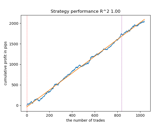
Figure 1. Testing the best model after sorting

The following model also turned out to be quite good and has a large number of trades:

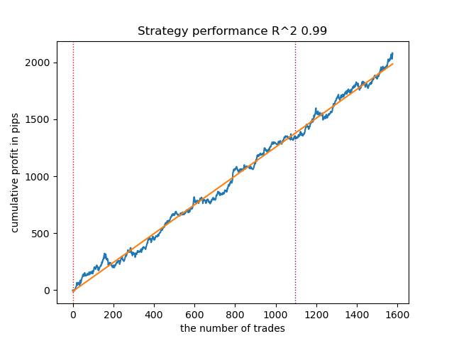
Figure 2. Testing the second-ranked model

Since the models are trained and tested very quickly, you can restart the loop many times to get the highest quality models. For example, after the next restart and sorting, we got this variant:

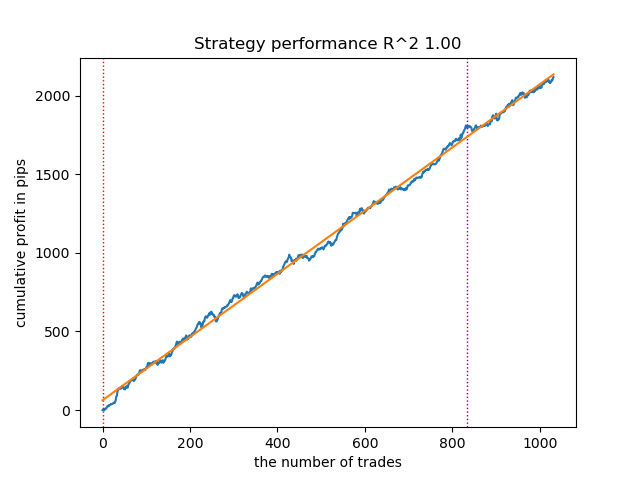
Figure 3. Testing the best model after repeated training loop

Training with moving averages and standard deviations

Let's change our features and see how the models perform.

def get_features(data: pd.DataFrame) -> pd.DataFrame:
    pFixed = data.copy()
    pFixedC = data.copy()
    count = 0

    for i in hyper_params['periods']:
        pFixed[str(count)] = pFixedC.rolling(i).mean()
        count += 1
    
    for i in hyper_params['periods_meta']:
        pFixed[str(count)+'meta_feature'] = pFixedC.rolling(i).std()
        count += 1

    return pFixed.dropna()

Simple moving averages will be used as the main features, and standard deviations will be used as meta-features.

Start the learning loop and consider the best models:

Iteration: 0, Cluster: 0
R2: 0.9312180471969619
Iteration: 0, Cluster: 1
R2: 0.9839766532391275
too few samples: 101
Iteration: 0, Cluster: 3
R2: 0.9643925934007344
too few samples: 299
Iteration: 0, Cluster: 5
R2: 0.9960009821184868
too few samples: 19
Iteration: 0, Cluster: 7
R2: 0.9557947960449501
Iteration: 0, Cluster: 8
R2: 0.9747160963596306
Iteration: 0, Cluster: 9
R2: 0.5526910449937035
Execution time:  2.8627688884735107

This is what the best model looks like in the tester:

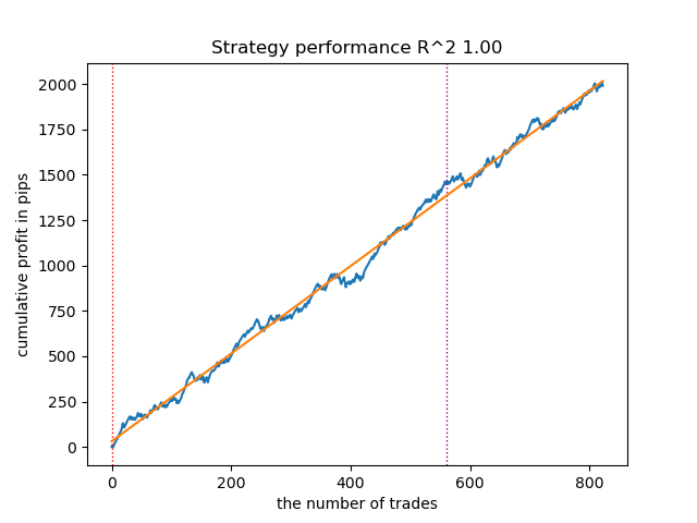
Figure 4. Testing the best model over moving averages

The second best model also shows a good result:

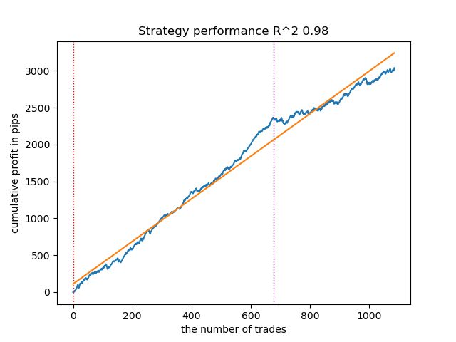
Figure 5. Testing the second model over moving averages

By restarting the training loop a few more times, I got a more accurate balance chart:

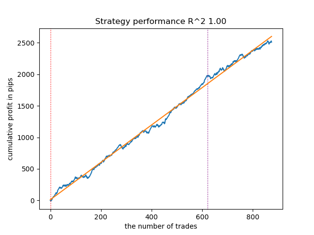
Figure 6. Testing the best model after repeated training loop

Here I have not experimented with the number of features (a list of their periods), so, in fact, it is possible to obtain a wide variety of such models. The screenshots provided simply demonstrate some of the variants.

Fighting against overfitting

It often happens that the excessive complexity of a model has a negative effect on its generalizing abilities. Even subject to the validation phase and the early stop. In this case, you can try to reduce the number of features and/or simplify the model. Complexity of the model in the CatBoost algorithm refers to the number of iterations or sequentially constructed decision trees. In fit_final_models() function try changing the following values:

def fit_final_models(clustered, meta) -> list:
    # features for model\meta models. We learn main model only on filtered labels 
    X, X_meta = clustered[clustered.columns[:-1]], meta[meta.columns[:-1]]
    X = X.loc[:, ~X.columns.str.contains('meta_feature')]
    X_meta = X_meta.loc[:, X_meta.columns.str.contains('meta_feature')]
    
    # labels for model\meta models
    y = clustered['labels']
    y_meta = meta['clusters']
    
    y = y.astype('int16')
    y_meta = y_meta.astype('int16')

    # train\test split
    train_X, test_X, train_y, test_y = train_test_split(
        X, y, train_size=0.8, test_size=0.2, shuffle=True)
    
    train_X_m, test_X_m, train_y_m, test_y_m = train_test_split(
        X_meta, y_meta, train_size=0.8, test_size=0.2, shuffle=True)


    # learn main model with train and validation subsets
    model = CatBoostClassifier(iterations=100,
                               custom_loss=['Accuracy'],
                               eval_metric='Accuracy',
                               verbose=False,
                               use_best_model=True,
                               task_type='CPU',
                               thread_count=-1)
    model.fit(train_X, train_y, eval_set=(test_X, test_y),
              early_stopping_rounds=15, plot=False)

Reduce the number of iterations to 100 and the early stop value to 15. This will allow you to build a less complex model.

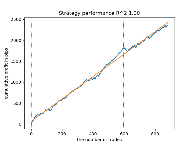
Figure 7. Testing a less "complex" model

Exporting models to the Meta Trader 5 terminal

The export_model_to_ONNX() function from export_lib() module contains the following strings:

# get features
    code += 'void fill_arays' + symbol + '_' + str(model_number) + '( double &features[]) {\n'
    code += '   double pr[], ret[];\n'
    code += '   ArrayResize(ret, 1);\n'
    code += '   for(int i=ArraySize(Periods'+ symbol + '_' + str(model_number) + ')-1; i>=0; i--) {\n'
    code += '       CopyClose(NULL,PERIOD_H1,1,Periods' + symbol + '_' + str(model_number) + '[i],pr);\n'
    code += '       ret[0] = MathMean(pr);\n'
    code += '       ArrayInsert(features, ret, ArraySize(features), 0, WHOLE_ARRAY); }\n'
    code += '   ArraySetAsSeries(features, true);\n'
    code += '}\n\n'

    # get features
    code += 'void fill_arays_m' + symbol + '_' + str(model_number) + '( double &features[]) {\n'
    code += '   double pr[], ret[];\n'
    code += '   ArrayResize(ret, 1);\n'
    code += '   for(int i=ArraySize(Periods_m' + symbol + '_' + str(model_number) + ')-1; i>=0; i--) {\n'
    code += '       CopyClose(NULL,PERIOD_H1,1,Periods_m' + symbol + '_' + str(model_number) + '[i],pr);\n'
    code += '       ret[0] = MathSkewness(pr);\n'
    code += '       ArrayInsert(features, ret, ArraySize(features), 0, WHOLE_ARRAY); }\n'
    code += '   ArraySetAsSeries(features, true);\n'
    code += '}\n\n'

The highlighted strings are responsible for calculating the features in the MQL5 code. In the event that you modify the features in the Python script in the get_features() function, as described above, you must alter their calculation in this code, or you can do this in an already exported .mqh file.

For example, in the exported XAUUSD_H1 ONNX include 0.mqh file, correct the following strings:

#include <Math\Stat\Math.mqh>
#resource "catmodel XAUUSD_H1 0.onnx" as uchar ExtModel_XAUUSD_H1_0[]
#resource "catmodel_m XAUUSD_H1 0.onnx" as uchar ExtModel2_XAUUSD_H1_0[]

int PeriodsXAUUSD_H1_0[10] = {5,35,65,95,125,155,185,215,245,275};
int Periods_mXAUUSD_H1_0[1] = {5};

void fill_araysXAUUSD_H1_0( double &features[]) {
   double pr[], ret[];
   ArrayResize(ret, 1);
   for(int i=ArraySize(PeriodsXAUUSD_H1_0)-1; i>=0; i--) {
       CopyClose(NULL,PERIOD_H1,1,PeriodsXAUUSD_H1_0[i],pr);
       ret[0] = MathStandardDeviation(pr);
       // ret[0] = MathMean(pr);
       ArrayInsert(features, ret, ArraySize(features), 0, WHOLE_ARRAY); }
   ArraySetAsSeries(features, true);
}

void fill_arays_mXAUUSD_H1_0( double &features[]) {
   double pr[], ret[];
   ArrayResize(ret, 1);
   for(int i=ArraySize(Periods_mXAUUSD_H1_0)-1; i>=0; i--) {
       CopyClose(NULL,PERIOD_H1,1,Periods_mXAUUSD_H1_0[i],pr);
       ret[0] = MathStandardDeviation(pr);
       ArrayInsert(features, ret, ArraySize(features), 0, WHOLE_ARRAY); }
   ArraySetAsSeries(features, true);
}

Now the calculation of features corresponds to the calculation of the get_features() function, which used only standard deviations. If moving averages were used, replace it with MathMean().

After compilation, we can test the bot already in Meta Trader 5.

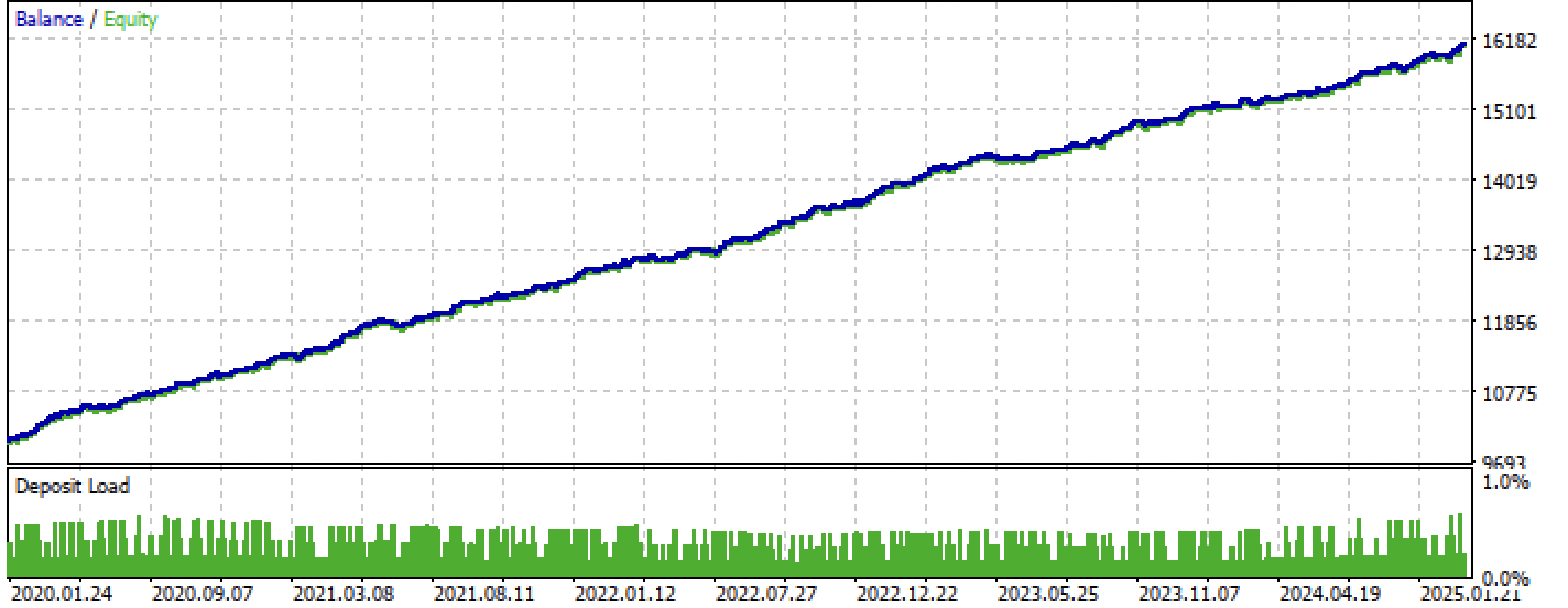
Figure 8. Testing on the training + forward interval

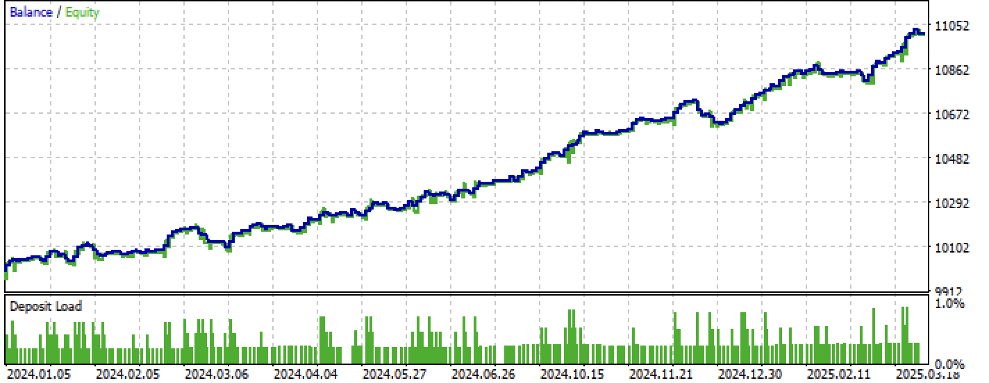
Figure 9. Testing only over the forward period

Conclusion

This article demonstrates another way to create unidirectional trend strategies, but based on clustering. The main difference of this approach is its intuitiveness and high learning rate. The quality of the resulting models is comparable to what was in the previous article.

 Python files.zip archive contains the following files for development in Python:

File name	Description
one direction clusters.py	The main script for learning models
labeling_lib.py	Updated module with trade markers
tester_lib.py	Updated custom tester for machine learning-based strategies
export_lib.py	A module to export models to the terminal
XAUUSD_H1.csv	The quotation file exported from the MetaTrader 5 terminal

 MQL5 files.zip archive contains files for MetaTrader 5:

File name	Description
one direction clusters.ex5	Compiled bot from this article
one direction clusters.mq5	The source of the bot from the article
folder Include//Trend following	Location of the ONNX models and the header file for connecting to the bot.