Data Science and ML (Part 43): Hidden Patterns Detection in Indicators Data Using Latent Gaussian Mixture Models (LGMM)

Contents
- Introduction
- What is a Latent Gaussian Mixture Model
- Mathematics behind LGMM
- Training LGMM on indicators data
- An MQL5 indicator based on LGMM
- Finding the best number of components for LGMM
- Latent Gaussian Mixture Model alongside a classifier model
- LGMM based trading robot
- Conclusion
Introduction
Almost all trading strategies available that we use as traders are based on some pattern identification and detection. We examine indicators for patterns and confirmations, and sometimes we even draw objects and lines, such as support and resistance lines, to identify the market's state.
While pattern detection is an easy task for us humans in financial markets, it is challenging to program and automate this process because of the nature of the markets (noisy and chaotic).
Some traders have adopted to the use of Artificial Intelligence (AI) and machine learning for this particular task using various computer vision-based techniques which process images data similar to what humans do, as we discussed in one of the previous articles.
In this article, we will discuss a probabilistic model named Latent Gaussian Mixture Model (LGMM), which is capable of detecting patterns. Given the indicators data, we will explore this model's effectiveness in detecting hidden patterns and making accurate predictions in the financial markets.

What is a Latent Gaussian Mixture Model (LGMM)?
Latent Gaussian Mixture Model is a probabilistic model that assumes data is generated from a mixture of multiple Gaussian distributions, each associated with a latent (hidden) variable.
It is an extension of the Gaussian Mixture Model (GMM) that incorporates latent variables that explain cluster assignment for each observation.
Latent Gaussian models are used to analyze data where the underlying processes generating the data are not directly observable and are assumed to have a Gaussian (normal) distribution.
The 'latent' part refers to these unobserved variables, much like the unseen electrical signals in a circuit, which influence the system's behavior but are not directly measured.
In financial markets, these latent variables can represent underlying trading patterns in the data that we often misinterpret or miss out.
Simply put, the backbone of LGMM involves:
- Latent Variables
These are unobserved variables assumed to be Gaussian, representing underlying factors that affect the observed data. - Observations
The actual data collected, which is typically non-Gaussian and may follow any distribution linked to the latent variables through a known function. - Parameters
These govern the relationship between latent variables and observations, including the means and variances of the distributions.
Mathematics behind LGMM
LGMM is a probabilistic generative model with a clustering technique at its core. It has:
Latent variables
- These are not directly observed
- They represent the component (cluster) from which a data point is drawn.
- They are often modeled as a categorical (discrete) distribution, e.g.,

The Mixture model
The probability distribution of the data is a weighted sum of several Gaussian distributions.

Where:
-
 is the mixing coefficient (prior probability) of a component
  ,
, 
-
 = Gaussian distribution with mean
  and covariance
Latent Variable Representation
Instead of modelling p(x) directly, we consider:
![]()
Where:
The Goal of this model is to estimate latent variables and the parameters ![]() .
.
The most common method used to determine these variables is the Expectation-Maximization (EM) algorithm.
Expectation-Maximization (EM) for LGMM
This involves two steps, Expectation and Minimization.
Step 01, Expectations.
This involves estimating the posterior probability that each data point belongs to each Gaussian.

Step 02, Maximization
This step involves updating the parameters using the ![]() .
.


In training, both step 01 and step 02 are repeated until the model converges.
LGMM has been used in several applications in the real world, such as clustering the data with uncertainty (soft clustering), in detecting anomalies, in density estimation, and in voice recognition-related tasks.
Training LGMM on Indicators Data
We know that inside the indicators data, there are patterns that, as traders, we use in making informed trading decisions. Our goal is to use LGMM to detect those patterns first.
We start by collecting indicators data from MetaTrader 5 first using MQL5 language.
- Symbol = XAUUSD.
- Timeframe = DAILY.
Filename: Get XAUUSD Data.mq5
#include <Arrays\ArrayString.mqh>
#include <Arrays\ArrayObj.mqh>
#include <pandas.mqh> //https://www.mql5.com/en/articles/17030

input datetime start_date = D'2005.01.01';
input datetime end_date = D'2023.01.01';

input string symbol = "XAUUSD";
input ENUM_TIMEFRAMES timeframe = PERIOD_D1;

struct indicator_struct
 {
   long handle;
   CArrayString buffer_names; //buffer_names array
 };

indicator_struct indicators[15]; //Structure for keeping indicator handle alongside its buffer names
//+------------------------------------------------------------------+
//| Script program start function                                    |
//+------------------------------------------------------------------+
void OnStart()
  {
//---

   vector time, open, high, low, close;
   if (!SymbolSelect(symbol, true))
      {
         printf("%s failed to select symbol %s, Error = %d",__FUNCTION__,symbol,GetLastError());
         return;
      }

 //---

   time.CopyRates(symbol, timeframe, COPY_RATES_TIME, start_date, end_date);
   open.CopyRates(symbol, timeframe, COPY_RATES_OPEN, start_date, end_date);
   high.CopyRates(symbol, timeframe, COPY_RATES_HIGH, start_date, end_date);
   low.CopyRates(symbol, timeframe, COPY_RATES_LOW, start_date, end_date);
   close.CopyRates(symbol, timeframe, COPY_RATES_CLOSE, start_date, end_date);

   CDataFrame df;

   df.insert("Time", time);
   df.insert("Open", open);
   df.insert("High", high);
   df.insert("Low", low);
   df.insert("Close", close);

//--- Oscillators

   indicators[0].handle = iATR(symbol, timeframe, 14);
   indicators[0].buffer_names.Add("ATR");

   indicators[1].handle = iBearsPower(symbol, timeframe, 13);
   indicators[1].buffer_names.Add("BearsPower");

   indicators[2].handle = iBullsPower(symbol, timeframe, 13);
   indicators[2].buffer_names.Add("BullsPower");

   indicators[3].handle = iChaikin(symbol, timeframe, 3, 10, MODE_EMA, VOLUME_TICK);
   indicators[3].buffer_names.Add("Chainkin");

   indicators[4].handle = iCCI(symbol, timeframe, 14, PRICE_OPEN);
   indicators[4].buffer_names.Add("CCI");

   indicators[5].handle = iDeMarker(symbol, timeframe, 14);
   indicators[5].buffer_names.Add("Demarker");

   indicators[6].handle = iForce(symbol, timeframe, 13, MODE_SMA, VOLUME_TICK);
   indicators[6].buffer_names.Add("Force");

   indicators[7].handle = iMACD(symbol, timeframe, 12, 26, 9, PRICE_OPEN);
   indicators[7].buffer_names.Add("MACD MAIN_LINE");
   indicators[7].buffer_names.Add("MACD SIGNAL_LINE");

   indicators[8].handle = iMomentum(symbol, timeframe, 14, PRICE_OPEN);
   indicators[8].buffer_names.Add("Momentum");

   indicators[9].handle = iOsMA(symbol, timeframe, 12, 26, 9, PRICE_OPEN);
   indicators[9].buffer_names.Add("OsMA");

   indicators[10].handle = iRSI(symbol, timeframe, 14, PRICE_OPEN);
   indicators[10].buffer_names.Add("RSI");

   indicators[11].handle = iRVI(symbol, timeframe, 10);
   indicators[11].buffer_names.Add("RVI MAIN_LINE");
   indicators[11].buffer_names.Add("RVI SIGNAL_LINE");

   indicators[12].handle = iStochastic(symbol, timeframe, 5, 3,3,MODE_SMA,STO_LOWHIGH);
   indicators[12].buffer_names.Add("StochasticOscillator MAIN_LINE");
   indicators[12].buffer_names.Add("StochasticOscillator SIGNAL_LINE");

   indicators[13].handle = iTriX(symbol, timeframe, 14, PRICE_OPEN);
   indicators[13].buffer_names.Add("TEMA");

   indicators[14].handle = iWPR(symbol, timeframe, 14);
   indicators[14].buffer_names.Add("WPR");

//--- Get buffers

   for (uint ind=0; ind<indicators.Size(); ind++) //Loop through all the indicators
      {
         for (uint buffer_no=0; buffer_no<(uint)indicators[ind].buffer_names.Total(); buffer_no++) //Their buffer names resemble their buffer numbers
            {
               string name = indicators[ind].buffer_names.At(buffer_no); //Get the name of the buffer, it is helpful for the DataFrame and CSV file

               vector buffer = {};
               if (!buffer.CopyIndicatorBuffer(indicators[ind].handle, buffer_no, start_date, end_date)) //Copy indicator buffer
                  {
                     printf("func=%s line=%d | Failed to copy %s indicator buffer, Error = %d",__FUNCTION__,__LINE__,name,GetLastError());
                     continue;
                  }

               df.insert(name, buffer); //Insert a buffer vector and its name to a dataframe object
            }
      }

   df.to_csv(StringFormat("Oscillators.%s.%s.csv",symbol,EnumToString(timeframe)), true); //Save all the data to a CSV file
  }
Outputs.
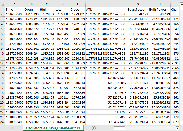
Notice that, we collected roughly all oscillator indicators which are built-in in MQL5, most of which happen to produce stationary data as they usually have minimum and maximum values. For example; The RSI indicator produces values between 0 and 100.
Despite the LGMM being capable of working with data of different statistical properties, such as non-stationary data. Stationary data makes it easier for LGMM to find meaningful structures and patterns because statistical properties of stationary data remains constant through time.
You are welcome to use any kind of data you'd prefer.
We collected Open, High, Low, Close, and Time (OHLCT) variables alongside indicators data for machine learning usage. This information can be used in visualization and in making the target variable for predictive machine learning models apart from LGMM.
Inside a Python script (Jupyter Notebook), the first thing we do is load this data shortly after importing the dependencies and initializing the MetaTrader 5 desktop app.
Filename: main.ipynb
import pandas as pd
import numpy as np
import MetaTrader5 as mt5
import os
from Trade.TerminalInfo import CTerminalInfo
import matplotlib.pyplot as plt
import seaborn
import warnings

warnings.filterwarnings("ignore")
seaborn.set_style("darkgrid")

if not mt5.initialize():
    print("Failed to Initialize MetaTrade5, Error = ",mt5.last_error())
    mt5.shutdown()


terminal = CTerminalInfo() # similarly to CTerminalInfo from MQL5. For getting information about the MetaTrader5 app
We Import the data from the common path (folder), which is where we saved it using MQL5.
common_path = os.path.join(terminal.common_data_path(), "Files")
symbol = "XAUUSD"
timeframe = "PERIOD_D1"

df = pd.read_csv(os.path.join(common_path, f"Oscillators.{symbol}.{timeframe}.csv")) # the same naming pattern as the one used in the MQL5 script

# Identify max float value
max_float = np.finfo(float).max

# Replace all max float (double) values with NaN produced by preliminary indicator calculations
df = df.replace(max_float, np.nan)
df.dropna(inplace=True)
df["Time"] = pd.to_datetime(df["Time"], unit="s")

df.head()
Outputs.
        Time    Open    High    Low     Close   ATR     BearsPower      BullsPower      Chainkin        CCI     ...     MACD SIGNAL_LINE        Momentum        OsMA    RSI     RVI MAIN_LINE   RVI SIGNAL_LINE StochasticOscillator MAIN_LINE  StochasticOscillator SIGNAL_LINE        TEMA    WPR
0       2005-01-03      438.45  438.71  426.72  429.55  5.481429        -12.314215      -0.324215       -1079.046551    -51.013015      ...     0.175727        99.870165       -0.582169       46.666555       -0.082596       0.018515        26.976532       32.920132       -0.000089       -85.144357
1       2005-01-04      429.52  430.18  423.71  427.51  5.450000        -13.677899      -7.207899       -1129.324384    -235.622347     ...     -0.000779       98.615544       -1.252741       37.393138       -0.158362       -0.048541       22.158658       27.150101       -0.000190       -82.774252
2       2005-01-05      427.50  428.77  425.10  426.58  5.162143        -10.743913      -7.073913       -1496.644248    -196.837418     ...     -0.247283       97.044402       -1.816758       35.666584       -0.227422       -0.119850       17.070979       22.068723       -0.000325       -86.990027
3       2005-01-06      426.31  427.85  420.17  421.37  5.234286        -13.606211      -5.926211       -3349.884147    -164.038728     ...     -0.576309       97.480164       -2.194161       34.651526       -0.269634       -0.187300       14.096364       17.775334       -0.000482       -95.312500
4       2005-01-07      421.39  425.48  416.57  419.02  5.605000        -15.098181      -6.188181       -4970.426959    -168.301515     ...     -1.015433       95.440750       -2.669414       30.754440       -0.305796       -0.243045       11.442611       14.203318       -0.000670       -91.609589
Let's prepare the target variable for a classification problem for later usage in classifier machine learning models. We drop non-indicator features along the way.
lookahead = 1

df["future_close"] = df["Close"].shift(-lookahead)
new_df = df.dropna()

new_df["Direction"] = np.where(new_df["future_close"]>new_df["Close"], 1, -1) # if a the close value in the next bar(s)=lookahead is above the current close price, thats a long signal otherwise that's a short signal
from sklearn.model_selection import train_test_split

X = new_df.drop(columns=[
    "Time",
    "Open",
    "High",
    "Low",
    "Close",
    "future_close",
    "Direction"
])

y = new_df["Direction"]

X_train, X_test, y_train, y_test = train_test_split(X, y, test_size=0.2, shuffle=True, random_state=42)
We have to check to ensure that we have the "indicators data" we need.
X_train.head()
Outputs.
        ATR     BearsPower      BullsPower      Chainkin        CCI     Demarker        MACD MAIN_LINE  MACD SIGNAL_LINE        Momentum        OsMA    RSI     RVI MAIN_LINE   RVI SIGNAL_LINE StochasticOscillator MAIN_LINE  StochasticOscillator SIGNAL_LINE        TEMA    WPR
1057    30.139286       34.958195       62.858195       16280.794393    268.371098      251356.076923   -1.759289       -15.645899      107.768519      13.886610       62.077386       0.229591        0.108028        92.301971       83.886543       -0.002663       -8.048595
3806    3.096429        0.724299        3.314299        -1279.189840    69.806094       696.923077      -0.121217       -0.952863       100.299538      0.831645        52.157089       0.096237        0.080054        67.031250       71.466497       -0.000077       -21.325052
38884   5.927143        -8.488258       -3.858258       -2005.866698    -213.672289     -3333.080000    -0.049837       0.496440        99.774916       -0.546277       39.550361       -0.022395       0.035070        28.046540       49.606252       0.000012        -73.130342
10351   2.060714        -0.491108       1.158892        723.246254      40.384615       2508.735385     1.293179        0.953618        100.533084      0.339561        58.791715       0.217352        0.294053        57.239819       69.770534       0.000123        -19.070322
38170   5.632143        -5.682364       -3.262364       -1321.008995    -109.039933     -1673.607692    -0.609996       0.785433        99.712893       -1.395429       41.917705       -0.062258       -0.053202       13.322009       9.490964        0.000035        -77.826942
Let's finally train LGMM .
from sklearn.mixture import GaussianMixture
from skl2onnx import convert_sklearn
from skl2onnx.common.data_types import FloatTensorType

components = 3

gmm = GaussianMixture(n_components=components, covariance_type="full", random_state=42)
gmm.fit(X_train)

latent_features_train = gmm.predict_proba(X_train)
latent_features_test = gmm.predict_proba(X_test)
I'm using 3 components for the Gaussian Mixture model, hoping it can cluster the patterns observed in the indicators between 3 clusters. Supposedly, one cluster for bullish trend (signal), the other cluster for bearish signal, and the other for consolidation or a ranging signal. Again, this is just a guess.
Similarly to other unsupervised machine learning and clustering techniques, it is difficult to interpret the resulting components (outcomes) produced by the model. For now, we can only assume that each one of the component belongs to the three classes I just described.
You might be wondering why I am calling the model a Latent Gaussian Mixture Model (LGMM), but I end up deploying a model named GaussianMixture from Scikit-Learn?
The imported GaussianMixture model has a functionality equivalent to the LGMM as described in the mathematics section of this post. These two are theoretically the same.
Let's print the latent_features_train array.
latent_features_train
Outputs.
array([[9.48947877e-13, 1.08107288e-62, 1.00000000e+00],
       [9.71935407e-01, 2.80542130e-02, 1.03801388e-05],
       [5.35722226e-03, 9.94642667e-01, 1.10916653e-07],
       ...,
       [7.72441751e-08, 8.80712550e-41, 9.99999923e-01],
       [9.99975623e-01, 1.07924534e-33, 2.43771745e-05],
       [1.91968188e-01, 8.08030586e-01, 1.22621110e-06]], shape=(3760, 3))
LGMM has produced an array of 3 elements on every row of predictions, each column representing the probability of the received data input belonging to one of the 3 clusters. The sum of probability for all 3 columns is equal to 1 on every row.
Since this is challenging to interpret as it stands, let's convert this model into ONNX format, visualize the clusters in MQL5, and see what conclusions we can draw upon the outputs produced by this probabilistic model.
An MQL5 Indicator Based on the Latent Gaussian Mixture Model (LGMM)
We start by saving LGMM to ONNX format.
# Define input type (shape should match your training data)
initial_type = [("float_input", FloatTensorType([None, X_train.shape[1]]))]

# Convert the pipeline to ONNX format
onnx_model = convert_sklearn(gmm, initial_types=initial_type)

# Save the model to a file
with open(os.path.join(common_path, f"LGMM.{symbol}.{timeframe}.onnx"), "wb") as f:
    f.write(onnx_model.SerializeToString())
Below is the model's architecture when opened in Netron.
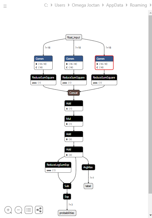
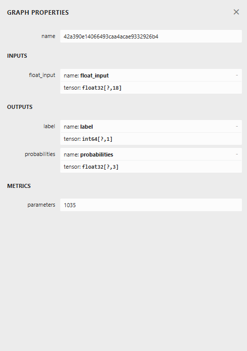
This model has a strange architecture with two outputs in the final node, one for the predicted label and the other for probabilities. We need to have this in mind when implementing the code for loading for this model in MQL5.
Loading LGMM in MQL5
Filename: Gaussian Mixture.mqh
We need the output structure that takes multiple arrays of values to accommodate two output nodes, each with an array of outputs.
class CGaussianMixture
  {
protected:

   bool initialized;
   long onnx_handle;
   void PrintTypeInfo(const long num,const string layer,const OnnxTypeInfo& type_info);

   ulong inputs[]; //Inputs of a model in dimensions [nxn]
   struct outputs_struct
    {
      ulong outputs[];
    } model_output_structure[];  //Outputs of the model structure array
Then.
bool CGaussianMixture::OnnxLoad(long &handle)
 {
//--- since not all sizes defined in the input tensor we must set them explicitly
//--- first index - batch size, second index - series size, third index - number of series (only Close)

   OnnxTypeInfo type_info; //Getting onnx information for Reference In case you forgot what the loaded ONNX is all about

   long input_count=OnnxGetInputCount(handle);
   if (MQLInfoInteger(MQL_DEBUG))
      Print("model has ",input_count," input(s)");

   for(long i=0; i<input_count; i++)
     {
      string input_name=OnnxGetInputName(handle,i);
      if (MQLInfoInteger(MQL_DEBUG))
         Print(i," input name is ",input_name);

      if(OnnxGetInputTypeInfo(handle,i,type_info))
        {
          if (MQLInfoInteger(MQL_DEBUG))
            PrintTypeInfo(i,"input",type_info);
          ArrayCopy(inputs, type_info.tensor.dimensions);
        }
     }

   long output_count=OnnxGetOutputCount(handle);
   if (MQLInfoInteger(MQL_DEBUG))
      Print("model has ",output_count," output(s)");

   ArrayResize(model_output_structure, (int)output_count);

   for(long i=0; i<output_count; i++)
     {
      string output_name=OnnxGetOutputName(handle,i);
      if (MQLInfoInteger(MQL_DEBUG))
         Print(i," output name is ",output_name);

      if(OnnxGetOutputTypeInfo(handle,i,type_info))
       {
         if (MQLInfoInteger(MQL_DEBUG))
            PrintTypeInfo(i,"output",type_info);

         ArrayCopy(model_output_structure[i].outputs, type_info.tensor.dimensions);
       }

       //--- Set the output shape

         replace(model_output_structure);
         if(!OnnxSetOutputShape(handle, i, model_output_structure[i].outputs))
          {
            if (MQLInfoInteger(MQL_DEBUG))
              {
                printf("Failed to set the Output[%d] shape Err=%d",i,GetLastError());
                DebugBreak();
              }

             return false;
          }
     }

//---

   replace(inputs);

//--- Setting the input size

   for (long i=0; i<input_count; i++)
     if (!OnnxSetInputShape(handle, i, inputs)) //Giving the Onnx handle the input shape
       {
         if (MQLInfoInteger(MQL_DEBUG))
           printf("Failed to set the input shape Err=%d",GetLastError());
         DebugBreak();
         return false;
       }


   initialized = true;
   if (MQLInfoInteger(MQL_DEBUG))
      Print("ONNX model Initialized");

   return true;
 }
//+------------------------------------------------------------------+
//|                                                                  |
//+------------------------------------------------------------------+
bool CGaussianMixture::Init(string onnx_filename, uint flags=ONNX_DEFAULT)
 {
   onnx_handle = OnnxCreate(onnx_filename, flags);

   if (onnx_handle == INVALID_HANDLE)
     return false;

   return OnnxLoad(onnx_handle);
 }
//+------------------------------------------------------------------+
//|                                                                  |
//+------------------------------------------------------------------+
bool CGaussianMixture::Init(const uchar &onnx_buff[], ulong flags=ONNX_DEFAULT)
 {
  onnx_handle = OnnxCreateFromBuffer(onnx_buff, flags); //creating onnx handle buffer

   if (onnx_handle == INVALID_HANDLE)
     return false;

  return OnnxLoad(onnx_handle);
 }
We made the predict method from this class to return two variables, the predicted label and a probability vector in a structure.
struct pred_struct
 {
   vector proba;
   long label;
 };
pred_struct CGaussianMixture::predict(const vector &x)
 {
   pred_struct res;

   if (!this.initialized)
    {
      if (MQLInfoInteger(MQL_DEBUG))
         printf("%s The model is not initialized yet to make predictions | call Init function first",__FUNCTION__);

      return res;
    }

//---

   vectorf x_float; //Convert inputs from a vector of double values to those float values
   x_float.Assign(x);

   vector label = vector::Zeros(model_output_structure[0].outputs[1]); //outputs[1] we get the second shape (columns) from an array
   vector proba = vector::Zeros(model_output_structure[1].outputs[1]); //outputs[1] we get the second shape (columns) from an array

   if (!OnnxRun(onnx_handle, ONNX_DATA_TYPE_FLOAT, x_float, label, proba)) //Run the model and get the predicted label and probability
     {
       if (MQLInfoInteger(MQL_DEBUG))
          printf("Failed to get predictions from Onnx err %d",GetLastError());

       DebugBreak();
       return res;
     }

//---

   res.label = (long)label[label.Size()-1]; //Get the last item available at the label's array
   res.proba = proba;

   return res;
 }
Let's call the predict function inside the main function of an indicator to provide us with latent features.
Filename: LGMM Indicator.mq5
int OnCalculate(const int32_t rates_total,
                const int32_t prev_calculated,
                const datetime &time[],
                const double &open[],
                const double &high[],
                const double &low[],
                const double &close[],
                const long &tick_volume[],
                const long &volume[],
                const int32_t &spread[])
  {
//--- Main calculation loop

   int lookback = 20;

   for (int i = prev_calculated; i < rates_total && !IsStopped(); i++)
   {
      if (i+1<lookback) //prevent data not found errors during copy buffer
         continue;

      int reverse_index = rates_total - 1 - i;

      //--- Get the indicators data

      vector x = getX(reverse_index, lookback);

      if (x.Size()==0)
         continue;

      pred_struct res = lgmm.predict(x);

      vector proba = res.proba;
      long label = res.label;

      ProbabilityBuffer[i] = proba.Max();

      // Determine color based on histogram value

      if (label == 0)
         ColorBuffer[i] = 0;
      else if (label == 1)
         ColorBuffer[i] = 1;
      else
         ColorBuffer[i] = 2;

      Comment("bars [",i+1,"/",rates_total,"]"," Proba: ",proba," label: ",label);
   }

//---
   return(rates_total);
  }
Inside the getX() function, we have to collect all indicator buffers in the same way as we did in the script when collecting the data for training.
vector getX(uint start=0, uint count=10)
 {
//--- Get buffers

   CDataFrame df;
   for (uint ind=0; ind<indicators.Size(); ind++) //Loop through all the indicators
      {
        uint buffers_total = indicators[ind].buffer_names.Total();

         for (uint buffer_no=0; buffer_no<buffers_total; buffer_no++) //Their buffer names resemble their buffer numbers
            {
               string name = indicators[ind].buffer_names.At(buffer_no); //Get the name of the buffer, it is helpful for the DataFrame and CSV file

               vector buffer = {};
               if (!buffer.CopyIndicatorBuffer(indicators[ind].handle, buffer_no, start, count)) //Copy indicator buffer
                  {
                     printf("func=%s line=%d | Failed to copy %s indicator buffer, Error = %d",__FUNCTION__,__LINE__,name,GetLastError());
                     continue;
                  }

               df.insert(name, buffer); //Insert a buffer vector and its name to a dataframe object
            }
      }

   return df.iloc(-1); //Return the latest information from the dataframe which is the most recent buffer
 }
Note: All indicators were initialized inside the Init function right after the model was initialized from the common folder, which is where we saved it using Python.
#include <Gaussian Mixture.mqh>
#include <Arrays\ArrayString.mqh>
#include <MALE5\Pandas\pandas.mqh>

CGaussianMixture lgmm;

input string symbol = "XAUUSD";
input ENUM_TIMEFRAMES timeframe = PERIOD_D1;

struct indicator_struct
 {
   long handle;
   CArrayString buffer_names;
 };

indicator_struct indicators[15];

//--- Indicator buffers

double ProbabilityBuffer[];
double ColorBuffer[];
double MaBuffer[];
//+------------------------------------------------------------------+
//| Custom indicator initialization function                         |
//+------------------------------------------------------------------+
int OnInit()
  {
//--- indicator buffers mapping

   Comment("");

   // Setting indicator properties
   SetIndexBuffer(0, ProbabilityBuffer, INDICATOR_DATA);
   SetIndexBuffer(1, ColorBuffer, INDICATOR_COLOR_INDEX);

   // Setting histogram drawing style
   PlotIndexSetInteger(0, PLOT_DRAW_TYPE, DRAW_COLOR_HISTOGRAM);

   // Set indicator labels
   IndicatorSetString(INDICATOR_SHORTNAME, "3-Color Histogram");
   IndicatorSetInteger(INDICATOR_DIGITS, _Digits);

//---

   string filename = StringFormat("LGMM.%s.%s.onnx",symbol, EnumToString(timeframe));
   if (!lgmm.Init(filename, ONNX_COMMON_FOLDER))
      {
         printf("%s Failed to initialize the GaussianMixture model (LGMM) in ONNX format file={%s}, Error = %d",__FUNCTION__,filename,GetLastError());
      }

//--- Oscillators

   indicators[0].handle = iATR(symbol, timeframe, 14);
   indicators[0].buffer_names.Add("ATR");

   //...
   //...
   //...

   indicators[14].handle = iWPR(symbol, timeframe, 14);
   indicators[14].buffer_names.Add("WPR");

   for (uint i=0; i<indicators.Size(); i++)
     if (indicators[i].handle==INVALID_HANDLE)
        {
          printf("%s Invalid %s handle, Error = %d",__FUNCTION__,indicators[i].buffer_names[0],GetLastError());
          return INIT_FAILED;
        }

//---
   return(INIT_SUCCEEDED);
  }
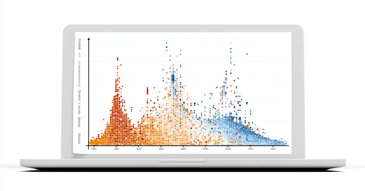
Finally, we run this indicator on the XAUUSD chart and the same timeframe that the model was trained on.
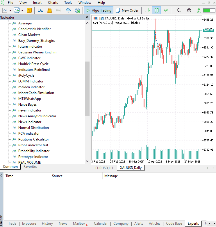
This indicator is still hard to interpret, but one pattern seems dominant, and that is the component presented in red color. It seems this pattern appears when the market is volatile (volatility is high) on either an uptrend or a downtrend. The remaining components are still not yet clear, this could be because we are not certain of the number of components we used for this model so, let us find the best number of components for this model.
Finding the Best Number of Components for LGMM
Since the Mixture Model offered by Scikit-Learn produces information criterion values, Akaike Information Criterion (AIC) and Bayesian Information Criterion (BIC). Let's plot these values against their component range in one plot and spot the elbow point(s).
The elbow point in a graph is a point where adding more components to the model results in only marginal improvement in performance, i.e,. the curve flattens.
Filename: main.ipynb
lowest_bic = np.inf
bic = []
aic = []
n_components_range = range(1, 10)

for n_components in n_components_range:
    gmm = GaussianMixture(n_components=n_components, random_state=42)
    gmm.fit(X)
    bic.append(gmm.bic(X_train))
    aic.append(gmm.aic(X_train))
    if bic[-1] < lowest_bic:
        best_gmm = gmm
        lowest_bic = bic[-1]

# Plot the BIC and AIC scores
plt.figure(figsize=(8, 5))
plt.plot(n_components_range, bic, label='BIC', marker='o')
plt.plot(n_components_range, aic, label='AIC', marker='o')
plt.xlabel('Number of components')
plt.ylabel('Score')
plt.title('LGMM selection: AIC vs BIC')
plt.legend()
plt.grid(True)
plt.show()
Outputs.

Both AIC and BIC curves drop sharply from 1 to 2 components and continue decreasing, but the rate of improvement slows down noticeably after 5 components for both. This means the best number of components that we should use for this model is 5.
Let's go back, retrain the model, and update the indicator.
Filename: main.ipynb
components = 5 # according to the elbow point

gmm = GaussianMixture(n_components=components, covariance_type="full", random_state=42)
gmm.fit(X_train)

latent_features_train = gmm.predict_proba(X_train)
latent_features_test = gmm.predict_proba(X_test)
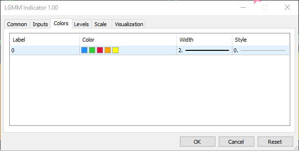
Now that we have 5 components inside of 3, meaning the model produces 5 probabilities that we can plot, we have to increase the number of colors in the indicator to 5 for the colored histogram and handle 5 different cases for the predicted labels.
Filename: LGMM Indicator.mq5
#property indicator_color1 clrDodgerBlue, clrLimeGreen, clrCrimson, clrOrange, clrYellow
Inside OnCalculate function.
int OnCalculate(const int32_t rates_total,
                const int32_t prev_calculated,
                const datetime &time[],
                const double &open[],
                const double &high[],
                const double &low[],
                const double &close[],
                const long &tick_volume[],
                const long &volume[],
                const int32_t &spread[])
  {
//--- Main calculation loop

   int lookback = 20;

   for (int i = prev_calculated; i < rates_total && !IsStopped(); i++)
   {
      if (i+1<lookback) //prevent data not found errors during copy buffer
         continue;

      //...
      //...
      //...

      // Determine color based on predicted label

      if (label == 0)
         ColorBuffer[i] = 0;
      else if (label == 1)
         ColorBuffer[i] = 1;
      else if (label == 2)
         ColorBuffer[i] = 2;
      else if (label == 3)
         ColorBuffer[i] = 3;
      else
         ColorBuffer[i] = 4;

      Comment("bars [",i+1,"/",rates_total,"]"," Proba: ",proba," label: ",label);
   }
The new indicator appearance.
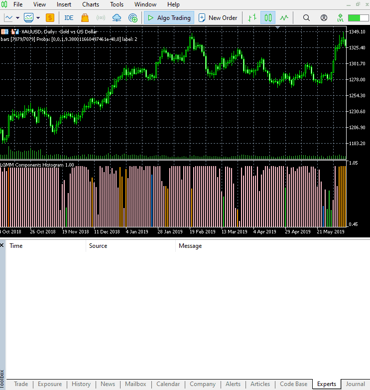
It looks great, but still difficult to read as we are often used to dealing with simple oscillators that often show oversold and overbought regions. Don't hesitate to explore this indicator and let us know your thoughts in the discussion section.
Now, let's use the LGMM alongside a machine learning model.
Latent Gaussian Mixture Model alongside a Classifier Model
We've now seen how we can use LGMM to produce latent features that represent the probability of a label belonging to a certain cluster, since it is difficult to understand these features. Let' use them in a Random forest classifier model alongside the indicator features hoping that this machine learning model can figure out how latent features affect the trading signals.
Filename: main.ipynb
We already created the target variable before when splitting the training and testing data, here it is again for reference.
from sklearn.model_selection import train_test_split

X = new_df.drop(columns=[
    "Time",
    "Open",
    "High",
    "Low",
    "Close",
    "future_close",
    "Direction"
])

y = new_df["Direction"]

X_train, X_test, y_train, y_test = train_test_split(X, y, test_size=0.2, shuffle=True, random_state=42)
After training the LGMM, we used it to make predictions on the training and testing data.
latent_features_train = gmm.predict_proba(X_train)
latent_features_test = gmm.predict_proba(X_test)
Since this data is difficult to read, let's add some feature names to it, making the features identifiable.
latent_features_train_df = pd.DataFrame(latent_features_train, columns=[f"LATENT_FEATURE_{i}" for i in range(latent_features_train.shape[1])])
latent_features_test_df = pd.DataFrame(latent_features_test, columns=[f"LATENT_FEATURE_{i}" for i in range(latent_features_test.shape[1])])
latent_features_train_df
Outputs.
| LATENT_FEATURE_0 | LATENT_FEATURE_1 | LATENT_FEATURE_2 | LATENT_FEATURE_3 | LATENT_FEATURE_4 | |
|---|---|---|---|---|---|
| 0 | 0.000000e+00 | 5.368039e-08 | 9.999999e-01 | 1.566000e-57 | 8.541983e-37 |
| 1 | 3.316692e-124 | 8.262106e-01 | 2.931424e-06 | 1.725415e-01 | 1.244990e-03 |
| 2 | 6.572730e-49 | 7.441120e-08 | 3.481699e-08 | 9.461818e-01 | 5.381811e-02 |
| 3 | 0.000000e+00 | 1.165057e-126 | 1.413762e-05 | 4.101964e-16 | 9.999859e-01 |
| 4 | 0.000000e+00 | 4.446778e-289 | 1.000000e+00 | 1.717945e-36 | 4.234123e-21 |
Let us stack these features alongside primary indicators data.
all_columns = X_train.columns.tolist() + latent_features_train_df.columns.tolist()

X_latent_train_arr = np.hstack([X_train, latent_features_train_df])
X_latent_test_arr = np.hstack([X_test, latent_features_test_df])

X_Train_latent = pd.DataFrame(X_latent_train_arr, columns=all_columns)
X_Test_latent = pd.DataFrame(X_latent_test_arr, columns=all_columns)

X_Train_latent.columns
Outputs.
Index(['ATR', 'BearsPower', 'BullsPower', 'Chainkin', 'CCI', 'Demarker',
       'Force', 'MACD MAIN_LINE', 'MACD SIGNAL_LINE', 'Momentum', 'OsMA',
       'RSI', 'RVI MAIN_LINE', 'RVI SIGNAL_LINE',
       'StochasticOscillator MAIN_LINE', 'StochasticOscillator SIGNAL_LINE',
       'TEMA', 'WPR', 'LATENT_FEATURE_0', 'LATENT_FEATURE_1',
       'LATENT_FEATURE_2', 'LATENT_FEATURE_3', 'LATENT_FEATURE_4'],
      dtype='object')
Let's pass this combined data to a random forest classifier.
from sklearn.ensemble import RandomForestClassifier
from sklearn.utils.class_weight import compute_class_weight

classes = np.unique(y_train)
weights = compute_class_weight(class_weight='balanced', classes=classes, y=y_train)

class_weights_dict = dict(zip(classes, weights))

params = {
    "n_estimators": 100,
    "min_samples_split": 2,
    "max_depth": 10,
    "max_leaf_nodes": 10,
    "criterion": "gini",
    "random_state": 42
}

model = RandomForestClassifier(**params, class_weight=class_weights_dict)

model.fit(X_Train_latent, y_train)
Model's evaluation.
y_train_pred = model.predict(X_Train_latent)

print("Train classification report\n", classification_report(y_train, y_train_pred))

y_test_pred = model.predict(X_Test_latent)

print("Test classification report\n", classification_report(y_test, y_test_pred))
Outputs.
Train classification report
               precision    recall  f1-score   support

          -1       0.60      0.67      0.63      1766
           1       0.68      0.61      0.64      1994

    accuracy                           0.64      3760
   macro avg       0.64      0.64      0.64      3760
weighted avg       0.64      0.64      0.64      3760

Test classification report
               precision    recall  f1-score   support

          -1       0.45      0.47      0.45       445
           1       0.50      0.48      0.49       495

    accuracy                           0.47       940
   macro avg       0.47      0.47      0.47       940
weighted avg       0.47      0.47      0.47       940
The resulting model has a bad performance on the validation sample, there is a lot we can do to improve it, but for now, let's observe the feature importance plot produced by the model.
importances = model.feature_importances_
feature_names = X_Train_latent.columns if hasattr(X_Train_latent, 'columns') else [f'feature_{i}' for i in range(X_Train_latent.shape[1])]

# Create DataFrame and sort
importance_df = pd.DataFrame({'feature': all_columns, 'importance': importances})
importance_df = importance_df.sort_values('importance', ascending=False)

# Plot
plt.figure(figsize=(8, 6))
plt.barh(importance_df['feature'], importance_df['importance'], color='red')
plt.title('RFC Feature Importance (Gini Importance)')
plt.xlabel('Importance Score')
plt.gca().invert_yaxis()  # Most important on top
plt.show()
Outputs.
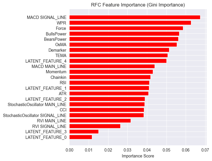
Latent features are proving to be important to the model, meaning they carry some patterns and information that contribute to the model's predictions.
The reason for this underperforming model might be due to the nature of the target variable deployed. The lookahead value of 1 might be wrong.
When using these indicators for making informed trading decisions, we don't usually use them to predict the next bar. For example, If the RSI value is below the threshold value of 30 (oversold) we can say that the market might undergo bulish for a couple of bars ahead. Not on the next bar only like the way we are currently training our model.
So let's re-create the target variable using the lookahead value of 5.
lookahead = 5

df["future_close"] = df["Close"].shift(-lookahead)
new_df = df.dropna()

new_df["Direction"] = np.where(new_df["future_close"]>new_df["Close"], 1, -1) # if a the close value in the next bar(s)=lookahead is above the current close price, thats a long signal otherwise that's a short signal
Now, evaluating the model on both training and validation data produces a different outcome.
Train classification report
               precision    recall  f1-score   support

          -1       0.56      0.70      0.62      1706
           1       0.69      0.54      0.61      2050

    accuracy                           0.61      3756
   macro avg       0.62      0.62      0.61      3756
weighted avg       0.63      0.61      0.61      3756

Test classification report
               precision    recall  f1-score   support

          -1       0.46      0.61      0.52       392
           1       0.63      0.48      0.55       548

    accuracy                           0.54       940
   macro avg       0.55      0.55      0.53       940
weighted avg       0.56      0.54      0.54       940
And a different feature importance plot.
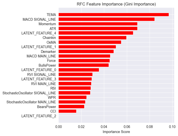
The model had an overall 54% accuracy, not a good one, but decent enough to make us believe what we are seeing on the feature importance plot.
Some of the latent features produced by the LGMM made it to the top of the most predictive features of the model.
The LATENT_FEATURE_4 being the 5th important feature to the Random forest classifier, the remaining latent features such as LATENT_FEATURE_0, and LATENT_FEATURE_1 did fairly well and surpased some raw indicators.
Overall, most features produced by LGMM have patterns beneficial to the classifier model.
Given this information, you now have a starting point for understanding the indicator.
The arrangement of the colors resembles the latent features.
LGMM-Based Trading Robot
Inside the Expert Advisor (EA), we start by importing necessary libraries.
Filename: LGMM BASED EA.mq5
#include <Random Forest.mqh>
#include <Arrays\ArrayString.mqh>
#include <pandas.mqh> //https://www.mql5.com/en/articles/17030
#include <Trade\Trade.mqh>
#include <Trade\PositionInfo.mqh>
#include <Trade\SymbolInfo.mqh>
#include <errordescription.mqh>

CSymbolInfo m_symbol;
CTrade m_trade;
CPositionInfo m_position;
CRandomForestClassifier rfc;
Again, we have to ensure that we are using the same symbol and timeframe as the one used in the training data.
#define MAGICNUMBER 11062025

input string SYMBOL = "XAUUSD";
input ENUM_TIMEFRAMES TIMEFRAME = PERIOD_D1;
input uint LOOKAHEAD = 5;
input uint SLIPPAGE = 100;
We initialize both models, the LGMM and the Random forest classifier model, inside the OnInit function.
int OnInit()
  {

   if (!MQLInfoInteger(MQL_DEBUG) && !MQLInfoInteger(MQL_TESTER))
    {
      ChartSetSymbolPeriod(0, SYMBOL, TIMEFRAME);
      if (!SymbolSelect(SYMBOL, true))
         {
            printf("%s failed to select SYMBOL %s, Error = %s",__FUNCTION__,SYMBOL,ErrorDescription(GetLastError()));
            return INIT_FAILED;
         }
    }

//--- Loading the Gaussian Mixture model

   string filename = StringFormat("LGMM.%s.%s.onnx",SYMBOL, EnumToString(TIMEFRAME));
   if (!lgmm.Init(filename, ONNX_COMMON_FOLDER))
      {
         printf("%s Failed to initialize the GaussianMixture model (LGMM) in ONNX format file={%s}, Error = %s",__FUNCTION__,filename,ErrorDescription(GetLastError()));
      }

//--- Loading the RFC model

   filename = StringFormat("rfc.%s.%s.onnx",SYMBOL,EnumToString(TIMEFRAME));
   Print(filename);
   if (!rfc.Init(filename, ONNX_COMMON_FOLDER))
      {
         printf("func=%s line=%d, Failed to Load the RFC in ONNX file={%s}, Error = %s",__FUNCTION__,__LINE__,filename,ErrorDescription(GetLastError()));
         return INIT_FAILED;
      }
//...
//... other lines of code
//...
}
Inside the getX function, we call LGMM to prepare latent features that can be used alongside the indicators data for final inputs of the Random forest classifier model.
vector getX(uint start=0, uint count=10)
 {
//--- Get buffers

   CDataFrame df;
   for (uint ind=0; ind<indicators.Size(); ind++) //Loop through all the indicators
      {
        uint buffers_total = indicators[ind].buffer_names.Total();

         for (uint buffer_no=0; buffer_no<buffers_total; buffer_no++) //Their buffer names resemble their buffer numbers
            {
               string name = indicators[ind].buffer_names.At(buffer_no); //Get the name of the buffer, it is helpful for the DataFrame and CSV file

               vector buffer = {};
               if (!buffer.CopyIndicatorBuffer(indicators[ind].handle, buffer_no, start, count)) //Copy indicator buffer
                  {
                     printf("func=%s line=%d | Failed to copy %s indicator buffer, Error = %d",__FUNCTION__,__LINE__,name,GetLastError());
                     continue;
                  }

               df.insert(name, buffer); //Insert a buffer vector and its name to a dataframe object
            }
      }

   if ((uint)df.shape()[0]==0)
      return vector::Zeros(0);

//--- predict the latent features

   vector indicators_data = df.iloc(-1); //index=-1 returns the last row from the dataframe which is the most recent buffer from all indicators

//--- Given the indicators let's predict the latent features

   vector latent_features = lgmm.predict(indicators_data).proba;

   if (latent_features.Size()==0)
      return vector::Zeros(0);

   return hstack(indicators_data, latent_features); //Return indicators data stacked alongside latent features
 }
Finally, we make a simple trading strategy that relies on trading signals produced by the random forest classifier model.
void OnTick()
  {
//--- Close trades after AI predictive horizon is over

   CloseTradeAfterTime(MAGICNUMBER, PeriodSeconds(TIMEFRAME)*LOOKAHEAD);

//--- Refresh tick information

   if (!m_symbol.RefreshRates())
     {
       printf("func=%s line=%s. Failed to copy rates, Error = %s",__FUNCTION__,ErrorDescription(GetLastError()));
       return;
     }

//---

    vector x = getX(); //Get all the input for the model

    if (x.Size()==0)
      return;

    long signal = rfc.predict(x).cls; //the class predicted by the random forest classifier
    double proba = rfc.predict(x).proba; //probability of the predictions

    double volume = m_symbol.LotsMin();

    if (!PosExists(POSITION_TYPE_SELL, MAGICNUMBER) && !PosExists(POSITION_TYPE_BUY, MAGICNUMBER)) //no position is open
      {
        if (signal == 1) //If a model predicts a bullish signal
          m_trade.Buy(volume, SYMBOL, m_symbol.Ask()); //Open a buy trade
        else if (signal == -1) // if a model predicts a bearish signal
          m_trade.Sell(volume, SYMBOL, m_symbol.Bid()); //open a sell trade
      }
  }
We close trades after a LOOKAHEAD number of bars have passed on the timeframe the model was trained on. LOOKAHEAD value needs to match the one used in making the target variable inside the training script.
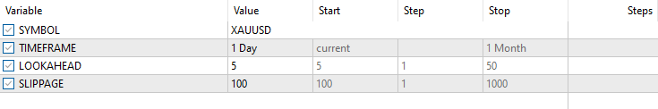
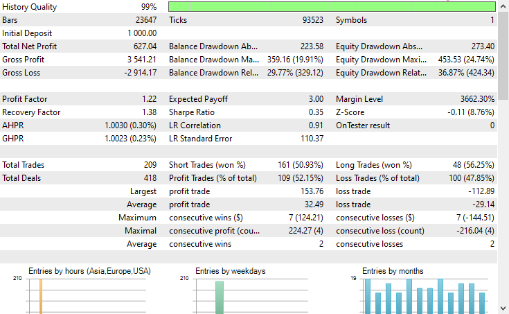
Tester configurations.
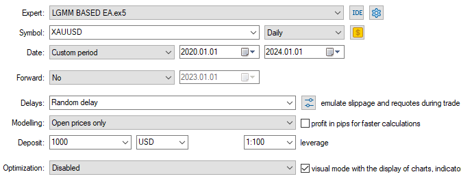
Inputs.
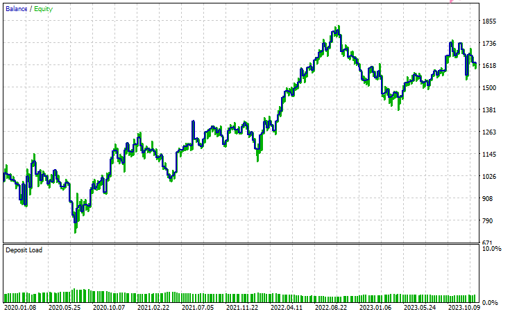
Tester Outcomes
Conclusion
Latent Gaussian Mixture Model (LGMM) is a decent technique that gives us meaningful features that comprise non-observable patterns that are often useful to machine learning models. However, just like any other machine learning models and predictive techniques, it has some drawback.
Latent Gaussian Mixture Model (LGMM): Overview
| Aspect | Description |
|---|---|
| What is LGMM | A method for extracting latent (hidden) features that represent non-observable patterns in data. These features can be useful for machine learning models. |
| Main Advantage | Captures meaningful hidden structures in data that can improve model performance. |
Limitations of LGMM
| Limitation | Explanation |
|---|---|
| Assumes Gaussian distribution | LGMM assumes each data point follows a multivariate normal distribution, which is rarely the case in financial data that tends to be chaotic and non-linear. |
| Sensitive to initialization | The model requires careful selection of the number of components. Poor initialization or wrong parameter choices can significantly reduce its effectiveness. |
| Hard to interpret results | The latent features it generates are difficult to understand or explain. As an unsupervised method, it doesn't label the patterns it detects, only clusters them. |
| Sensitive to outliers | Gaussian distributions are not robust to outliers. A few extreme values can skew the mean and inflate the variance, distorting the model's results. |
This model is the most useful when it comes to dimension reduction (reducing the number of features into a few meaningful ones) and for introducing new features to enrich the model with more useful information. I believe it is best to use it this way.
Best regards.
Stay tuned and contribute to machine learning algorithms development for the MQL5 language in this GitHub repository.
Attachments Table
| Filename | Description & Usage |
|---|---|
| Include\errordescription.mqh | Contains the description of all error codes produced by MetaTrader 5 in MQL5 language. |
| Include\Gaussian Mixture.mqh | A library which contains the class for initializing and deploying the Gaussian Mixture model stored in ONNX format. |
| Include\pandas.mqh | Contains a class for data storage and manipulation similar to Pandas offered in the Python programming language. |
| Include\Random Forest.mqh | A library which contains the class for initializing and deploying the random forest classifier stored in ONNX format. |
| Indicators\LGMM Indicator.mq5 | An indicator for displaying latent features produced by the Latent Gaussian Mixture Model (LGMM). |
| Scripts\Get XAUUSD Data.mq5 | A script for collecting oscillator indicators alongside OHLCT values from MetaTrader 5 and storing them to a CSV file. |
| Experts\LGMM BASED EA.mq5 | An Expert Advisor (EA) that opens and closes trades based on the predictions offered by the random forest classifier using the data, which is the combination of latent features produced by LGMM and oscillator indicators. |
| Python Code\main.ipynb | A Jupyter notebook (Python script) for data analysis, machine learning model training, etc. |
| Python Code\Trade\TerminalInfo.py | It has a class similar to CTerminalInfo provided in MQL5 for getting information about the selected MetaTrader 5 desktop app. |
| Python\requirements.txt | Has all the Python dependencies and their version numbers used in this project. |
| Common\Files\* | Has a sample CSV which contains training data and a couple of ONNX model files used in this article, only for reference. |
Warning: All rights to these materials are reserved by MetaQuotes Ltd. Copying or reprinting of these materials in whole or in part is prohibited.
This article was written by a user of the site and reflects their personal views. MetaQuotes Ltd is not responsible for the accuracy of the information presented, nor for any consequences resulting from the use of the solutions, strategies or recommendations described.

- Free trading apps
- Over 8,000 signals for copying
- Economic news for exploring financial markets
You agree to website policy and terms of use