
Reimagining Classic Strategies (Part 13): Taking Our Crossover Strategy to New Dimensions (Part 2)

In our last discussion on moving average crossovers, we examined how to minimize the inherent lag associated with moving averages. Moving average crossovers are well known for generating delayed signals. We shared that by fixing the periods of both moving averages to a common value—for example, a period of three as used in our previous discussion—we can obtain much more responsive trading signals. This improvement arises from applying moving average indicators separately to the open and close prices, even though they share the same period. By placing them on different price levels, we are still guaranteed to observe crossovers between the open and close moving averages. At the same time, this approach reduces the lag in the system by using short periods, typically smaller than five.
We demonstrated that this strategy offers advantages over the classical moving average crossover approach. In our initial discussion, we compared this new proposed crossover strategy against its classical counterpart. In this article, we will continue to advance our moving average crossover strategy and attempt to further reduce the inherent lag by exploring whether it is possible to forecast crossovers before they occur. This would enable us to trade proactively and respond more quickly to trading opportunities. Unlike typical market participants who wait for confirmation and react only after the crossover becomes apparent, we aim to build statistical models capable of detecting crossovers in advance, allowing us to position our accounts appropriately before the moves unfold.
Although detecting trading signals amidst market noise can be challenging, several data science principles can help strengthen our strategy. For example, we reference a presentation by the NASA Jet Propulsion Laboratory team at the California Institute of Technology (Caltech), which offers valuable insights. The link to the presentation is available here. This presentation focused on big data and introduced a key principle relevant to our discussion. Interested readers are encouraged to review the slides for themselves. Briefly, the principle states that certain challenging problems in data science can become easier to solve when projected into higher-dimensional spaces. For the reader's convenience, we have included an excerpt from the original presentation that is relevant for our discussion in Figure 1, below.
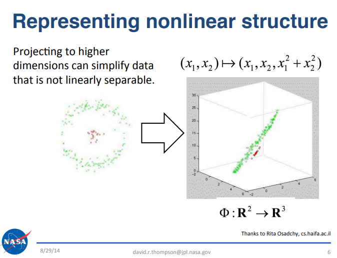
Figure 1: The slide above was originally part of the publicly available 'Big Data Analytics' presentation made by the NASA JPL team at Caltech University, September 2014.
For example, consider a dataset with three features, where the goal is to classify bullish and bearish market days. Achieving high classification accuracy may be difficult in this low 3-dimensional space. However, by projecting the dataset into higher dimensions, performance can improve because some problems become more separable in higher-dimensional feature spaces. Although machine learning does not guarantee success in all cases, this approach often yields better results and is often worth the check.
This principle contrasts with our previous discussions in our related series of articles, such as Self Optimizing Expert Advisors in MQL5, where we explored the benefits of dimensionality reduction techniques such as UMAP to reduce datasets from 30 features down to four. Typically, we focus on reducing dimensionality to simplify models and improve generalization. Today, however, we will take the opposite approach and deliberately increase the dimensionality of our dataset, as this may have practical value that we will demonstrate.
In this article, we will derive a manually handcrafted method for generating many new feature columns. In future discussions, we will work with more flexible algorithmic techniques for feature generation.
Getting Started in MQL5
To begin, we will first build a script to fetch all the necessary data from our MetaTrader 5 terminal. We will start by fixing certain constants relevant to our discussion. For example, the period for all moving averages will be set to a fixed value, and we will use simple moving averages throughout this discussion.
//+------------------------------------------------------------------+
//|                                                      ProjectName |
//|                                      Copyright 2020, CompanyName |
//|                                       http://www.companyname.net |
//+------------------------------------------------------------------+
#property copyright "Copyright 2024, MetaQuotes Ltd."
#property link      "https://www.mql5.com"
#property version   "1.00"
#property script_show_inputs

//--- Define our moving average indicator
#define MA_PERIOD 2                 //--- Moving Average Period
#define MA_TYPE   MODE_SMA          //--- Type of moving average we have
#define HORIZON   5                 //--- Forecast horizon
Additionally, we will define global variables such as handlers and buffers for the moving average indicators.
//--- Our handlers for our indicators
int ma_handle,ma_o_handle,ma_h_handle,ma_l_handle;

//--- Data structures to store the readings from our indicators
double ma_reading[],ma_o_reading[],ma_h_reading[],ma_l_reading[];

//--- File name
string file_name = Symbol() + " Market Data As Series Moving Average.csv";

//--- Amount of data requested
input int size = 3000;
Next, we proceed to define the main body of our script. When the script is executed, we will initialize our moving average handlers and then copy the values from these handlers into their associated buffers. As we prepare to write the data to a file, it is important to note that there are numerous columns to be filled. The first eight columns are standard: open, high, low, close prices, and their corresponding moving averages. Beyond these, we include columns representing the growth occurring within each price feed.
Furthermore, there are columns dedicated to calculating the relative changes between different price levels. For instance, in addition to calculating the change in the open price compared to its historical value, we also calculate the change in the open price relative to the close price, the change in the open price relative to the low price, and so forth. The same calculations are repeated for the moving averages. Altogether, this process generates 40 columns in our dataset. Finally, we store the actual values we intend to write and then close the file handler.
//+------------------------------------------------------------------+
//| Our script execution                                             |
//+------------------------------------------------------------------+
void OnStart()
  {
  int fetch = size + (HORIZON * 2);
//---Setup our technical indicators
   ma_handle = iMA(_Symbol,PERIOD_CURRENT,MA_PERIOD,0,MA_TYPE,PRICE_CLOSE);
   ma_o_handle = iMA(_Symbol,PERIOD_CURRENT,MA_PERIOD,0,MA_TYPE,PRICE_OPEN);
   ma_h_handle = iMA(_Symbol,PERIOD_CURRENT,MA_PERIOD,0,MA_TYPE,PRICE_HIGH);
   ma_l_handle = iMA(_Symbol,PERIOD_CURRENT,MA_PERIOD,0,MA_TYPE,PRICE_LOW);

//---Set the values as series
   CopyBuffer(ma_handle,0,0,fetch,ma_reading);
   ArraySetAsSeries(ma_reading,true);
   CopyBuffer(ma_o_handle,0,0,fetch,ma_o_reading);
   ArraySetAsSeries(ma_o_reading,true);
   CopyBuffer(ma_h_handle,0,0,fetch,ma_h_reading);
   ArraySetAsSeries(ma_h_reading,true);
   CopyBuffer(ma_l_handle,0,0,fetch,ma_l_reading);
   ArraySetAsSeries(ma_l_reading,true);

//---Write to file
   int file_handle=FileOpen(file_name,FILE_WRITE|FILE_ANSI|FILE_CSV,",");

   for(int i=size;i>=1;i--)
     {
      if(i == size)
        {
         FileWrite(file_handle,"Time",
                              //--- OHLC
                              "True Open",
                              "True High",
                              "True Low",
                              "True Close",
                              //--- MA OHLC
                              "True MA C",
                              "True MA O",
                              "True MA H",
                              "True MA L",
                              //--- Growth in OHLC
                              "Diff Open",
                              "Diff High",
                              "Diff Low",
                              "Diff Close",
                              //--- Growth in MA OHLC
                              "Diff MA Close 2",
                              "Diff MA Open 2",
                              "Diff MA High 2",
                              "Diff MA Low 2",
                              //--- Grwoth between channels
                              "O - C",
                              "Delta O - C",
                              "O - L",
                              "Delta O - L",
                              "O - H",
                              "Delta O - H",
                              "H - L",
                              "Delta H - L",
                              "C - H",
                              "Delta C - H",
                              "C - L",
                              "Delta C - L",
                              //--- Grwoth between MA channels
                              "MA O - C",
                              "MA Delta O - C",
                              "MA O - L",
                              "MA Delta O - L",
                              "MA O - H",
                              "MA Delta O - H",
                              "MA H - L",
                              "MA Delta H - L",
                              "MA C - H",
                              "MA Delta C - H",
                              "MA C - L",
                              "MA Delta C - L"
                  );
        }

      else
        {
         FileWrite(file_handle,
                   iTime(_Symbol,PERIOD_CURRENT,i),
                   //--- OHLC
                   iOpen(_Symbol,PERIOD_CURRENT,i),
                   iHigh(_Symbol,PERIOD_CURRENT,i),
                   iLow(_Symbol,PERIOD_CURRENT,i),
                   iClose(_Symbol,PERIOD_CURRENT,i),
                   //--- MA OHLC
                   ma_reading[i],
                   ma_o_reading[i],
                   ma_h_reading[i],
                   ma_l_reading[i],
                   //--- Growth in OHLC
                   iOpen(_Symbol,PERIOD_CURRENT,i)   - iOpen(_Symbol,PERIOD_CURRENT,(i + HORIZON)),
                   iHigh(_Symbol,PERIOD_CURRENT,i)   - iHigh(_Symbol,PERIOD_CURRENT,(i + HORIZON)),
                   iLow(_Symbol,PERIOD_CURRENT,i)    - iLow(_Symbol,PERIOD_CURRENT,(i + HORIZON)),
                   iClose(_Symbol,PERIOD_CURRENT,i)  - iClose(_Symbol,PERIOD_CURRENT,(i + HORIZON)),
                   //--- Growth in MA OHLC
                   ma_reading[i] - ma_reading[(i + HORIZON)],
                   ma_o_reading[i] - ma_o_reading[(i + HORIZON)],
                   ma_h_reading[i] - ma_h_reading[(i + HORIZON)],
                   ma_l_reading[i] - ma_l_reading[(i + HORIZON)],
                   //--- Growth between channels
                   iOpen(_Symbol,PERIOD_CURRENT,i) - iClose(_Symbol,PERIOD_CURRENT,i),
                   iOpen(_Symbol,PERIOD_CURRENT,i + HORIZON) - iClose(_Symbol,PERIOD_CURRENT,i + HORIZON),
                   iOpen(_Symbol,PERIOD_CURRENT,i) - iLow(_Symbol,PERIOD_CURRENT,i),
                   iOpen(_Symbol,PERIOD_CURRENT,i + HORIZON) - iLow(_Symbol,PERIOD_CURRENT,i + HORIZON),
                   iOpen(_Symbol,PERIOD_CURRENT,i) - iHigh(_Symbol,PERIOD_CURRENT,i),
                   iOpen(_Symbol,PERIOD_CURRENT,i + HORIZON) - iHigh(_Symbol,PERIOD_CURRENT,i + HORIZON),
                   iHigh(_Symbol,PERIOD_CURRENT,i) - iLow(_Symbol,PERIOD_CURRENT,i),
                   iHigh(_Symbol,PERIOD_CURRENT,i + HORIZON) - iLow(_Symbol,PERIOD_CURRENT,i + HORIZON),
                   iClose(_Symbol,PERIOD_CURRENT,i)  -  iHigh(_Symbol,PERIOD_CURRENT,i),
                   iClose(_Symbol,PERIOD_CURRENT,i + HORIZON)  -  iHigh(_Symbol,PERIOD_CURRENT,i + HORIZON),
                   iClose(_Symbol,PERIOD_CURRENT,i)  -  iLow(_Symbol,PERIOD_CURRENT,i),
                   iClose(_Symbol,PERIOD_CURRENT,i + HORIZON)  -  iLow(_Symbol,PERIOD_CURRENT,i + HORIZON),
                   //--- Growth between moving average channels
                   ma_o_reading[i] - ma_reading[i],
                   ma_o_reading[(i + HORIZON)] -  ma_reading[(i + HORIZON)],
                   ma_o_reading[i] -  ma_l_reading[i],
                   ma_o_reading[(i + HORIZON)] - ma_l_reading[(i + HORIZON)],
                   ma_o_reading[i] -  ma_h_reading[i],
                   ma_o_reading[(i + HORIZON)] - ma_h_reading[(i + HORIZON)],
                   ma_h_reading[i] - ma_l_reading[i],
                   ma_h_reading[(i + HORIZON)] - ma_l_reading[(i + HORIZON)],
                   ma_reading[i] -  ma_h_reading[i],
                   ma_reading[(i + HORIZON)] - ma_h_reading[(i + HORIZON)],
                   ma_reading[i] -  ma_l_reading[i],
                   ma_reading[(i + HORIZON)] - ma_l_reading[(i + HORIZON)]
                   );
        }
     }
//--- Close the file
   FileClose(file_handle);
  }
//+------------------------------------------------------------------+
Analyzing Our Data in Python
Now that you have finished deploying your script to the terminal and extracting the required data, we can begin analyzing and processing the data. First, we will load the standard libraries for numerical analysis.
import pandas as pd
import numpy as np
import seaborn as sns
import matplotlib.pyplot as plt
Next, we will read in the datasets. As you will notice, the dataset is of considerable width, and some columns have been truncated from view.
data = pd.read_csv("C:\\Users\\Westwood\\AppData\\Roaming\\MetaQuotes\\Terminal\\D0E8209F77C8CF37AD8BF550E51FF075\\MQL5\\Files\\EURUSD Market Data As Series Moving Average.csv")
data 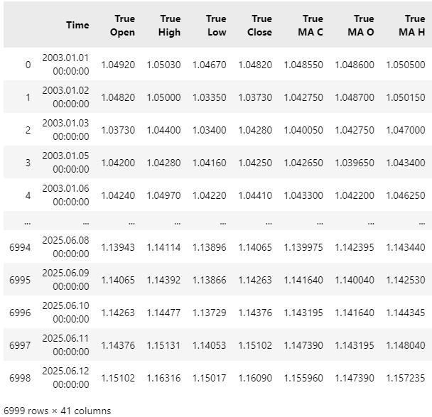
Figure 2: Visualizing the data we fetched from our MetaTrader 5 terminal.
We will then define our target variable. Recall that for this example, the target is the crossover between moving averages. A straightforward method to track this crossover is to monitor the midpoint between the two moving averages. By observing whether the midpoint has risen or fallen, we effectively capture the same information for our statistical models.
HORIZON             = 10

#Classical Target
data['Target']      =  0

#High Low Mid Point Target
data['Target 2']    = 0

#Open Close Mid Point Target
data['Target 3']    = 0

data.loc[data['True Close'].shift(-HORIZON) > data['True Close'],'Target'] = 1

#The Mid Point Between The High And The Low Moving Average
data.loc[((data['True MA H'].shift(-HORIZON) + data['True MA L'].shift(-HORIZON)) / 2) > ((data['True MA H'] + data['True MA L']) / 2),'Target 2'] = 1

#The Open And Close Mid Point
data.loc[((data['True MA O'].shift(-HORIZON) + data['True MA C'].shift(-HORIZON)) / 2) > ((data['True MA O'] + data['True MA C']) / 2),'Target 3'] = 1

data = data.iloc[:-HORIZON,:]
Before proceeding further, I would like to provide a brief demonstration illustrating the value of projecting datasets into higher dimensions. This will serve as a simple proof for readers who may be unfamiliar with this principle, ensuring we are all on the same page. We will start by creating a copy of the original dataset containing only the standard four columns: open, high, low, and close prices. Afterward, we will recalculate our target variable on this reduced dataset.
#Copy the dataset
X = data.iloc[:,:5].copy()
X['Target'] = data['True Close'].shift(-HORIZON) - data['True Close']
X.dropna(inplace=True)
Next, we will define a function that takes a dataset and appends an arbitrary number of columns filled with zeros. For example, if we call this function with our dataset copy and specify five columns, it will return the dataset with five additional columns, each filled with zeros.
def fill_zeros(f_data,f_n):
    #Copy the original data
    res = f_data.copy()

    #We want to keep the target at the end
    t = 'Target'
    v = res.pop('Target')

    #Add columns of zeros
    for i in np.arange(f_n):
        name = str(i) + ' Col'
        res[name] = 0

    #Place the target back
    res[t]= v

    #Return the new dataframe
    return(res)
We will then conduct a simple test by cross-validating our model with an increasing number of zero-filled columns and observe the effect on the cross-validation error. Note that the resulting graph is not smooth, indicating variability in the error as dimensions increase.
However, it is clear that the graph reaches new lows that it was unable to achieve earlier in the plot. At the very beginning, we observe the error level of our model when no additional zero-filled columns are present. As the number of zero columns increases, the error generally spikes and then falls to new lows, previously unattained. This observation should prompt the reader to question why the model’s performance improves despite no additional information being provided, remember that the zero columns contain no useful data for the model.
#Load our libraries
from sklearn.neural_network import MLPRegressor
from sklearn.model_selection import cross_val_score,TimeSeriesSplit

tscv = TimeSeriesSplit(n_splits=5,gap=HORIZON)
EPOCHS = 50

#Observe what happens to our error levels as we increase the number of columns in the dataset
res = []

for i in np.arange(EPOCHS):
    #Fetch new data with addtional columns of zeros
    new_data = fill_zeros(X,(1+i))

    #Record the new error
    res.append(np.mean(np.abs(cross_val_score(MLPRegressor(hidden_layer_sizes=(new_data.iloc[:,1:-1].shape[1],2,50,100),random_state=0,shuffle=False),X.iloc[:,1:-1],X.iloc[:,-1],cv=tscv,n_jobs=-1))))

plt.plot(res,color='black')
plt.grid()
plt.ylabel('RMSE Error')
plt.xlabel('Additional Columns of Zero')
plt.title('Our Error Levels Can Fall Without Any New Information')
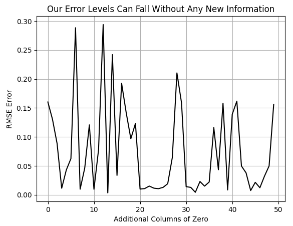
Figure 3: Our model's error levels fall even though we aren't providing any additional information.
There are several plausible explanations for this phenomenon. For the purpose of this discussion, we will adopt the perspective that increasing dimensionality has intrinsic value. We interpret this as evidence supporting the benefit of projecting data into higher-dimensional spaces. Although valid alternative explanations do exist, as far as we are concerned in our discussion this observation serves as motivation for the 32 handcrafted feature columns we created for our dataset. We believe that by increasing the number of additional columns, we can again achieve new lows in error. However, this time, instead of adding zeros, we intend to add meaningful information.
With our motivation established, we now proceed to identify our input and output columns. We first gather all input columns and store them in a variable named X.
X = data.iloc[:,1:-4].columns
Next, we list our target variables.
y2 = data['Target 2']
We will also need to define a function that returns a fresh instance of our statistical model.
return(RandomForestClassifier(random_state=0,n_estimators=500,max_depth=3,min_samples_leaf=20))
We then exclude any data overlapping with the back test period, as we do not want to overfit the model to all available data. It is important to reserve some data exclusively for testing. Folflowing this, we standardize and scale our dataset by subtracting the column means and dividing by the column standard deviations for each of the 40 columns. This process yields a scaled dataset.
data = data.iloc[:-(365*2),:]

Z = pd.DataFrame(columns=['Z1','Z2'])

Z['Z1'] = data.loc[:,X].mean()
Z['Z2'] = data.loc[:,X].std()

data.loc[:,X] = (data.loc[:,X] - data.loc[:,X].mean()) / data.loc[:,X].std()
Finally, we fit our model to all the training data before preparing to export the model in ONNX format, enabling its use within MQL5.
import onnx
from skl2onnx import convert_sklearn
from skl2onnx.common.data_types import FloatTensorType
from sklearn.ensemble import GradientBoostingRegressor

model = GradientBoostingRegressor(random_state=0,max_depth=3)
model.fit(data.loc[:,X],data.loc[:,'Target 2'])

initial_types = [("FLOAT INPUT",FloatTensorType([1,len(X)]))]

model_proto = convert_sklearn(model,initial_types=initial_types,target_opset=12)

onnx.save(model_proto,"EURUSD GBR PRICE D1.onnx")
Bringing it Altogether
We are now ready to begin assembling our Expert Advisor. Our first task is to define global constants that are not intended to change. Note that many of these definitions are the same as those established earlier in our data-fetching script. Specifically, the moving average period and the moving average type remain fixed to the same values. Additionally, we have defined the duration for holding each position, as well as the timeframe on which we will be trading.
//+------------------------------------------------------------------+
//| System constants                                                 |
//+------------------------------------------------------------------+
//--- Define our moving average indicator
#define MA_PERIOD 2                             //Moving Average Period
#define MA_TYPE   MODE_SMA                      //Type of moving average we have
#define HORIZON   10                            //Forecast horizon
#define TF PERIOD_D1
Next, we declare important global variables. For example, the Z1 and Z2 scores used to standardize and scale our dataset must be maintained within the Expert Advisor. We also require global variables for the moving average handlers and their corresponding buffers.
//+------------------------------------------------------------------+
//| Global definitions                                               |
//+------------------------------------------------------------------+
float Z1[] =
  {
   1.23933432e+00,  1.24403263e+00,  1.23474846e+00,  1.23936216e+00,
   1.23935910e+00,  1.23933128e+00,  1.24402971e+00,  1.23474522e+00,
   3.83991053e-05,  3.60920275e-05,  3.66240614e-05,  3.55759706e-05,
   3.68749001e-05,  3.98194600e-05,  3.78958300e-05,  3.79070139e-05,
   -2.78415082e-05, -3.06646429e-05,  4.58586036e-03,  4.58408532e-03,
   -4.69831123e-03, -4.70061831e-03,  9.28417159e-03,  9.28470363e-03,
   -4.67046972e-03, -4.66995367e-03,  4.61370187e-03,  4.61474996e-03,
   -2.78151462e-05, -3.07597060e-05,  4.58606247e-03,  4.58415002e-03,
   -4.69842067e-03, -4.70034430e-03,  9.28448314e-03,  9.28449433e-03,
   -4.67060553e-03, -4.66958460e-03,  4.61387762e-03,  4.61490973e-03
  };

float Z2[]=
  {
   0.12576155, 0.12640182, 0.125071, 0.12572605, 0.12568469,
   0.125719, 0.12636385, 0.12503521, 0.0150256, 0.01494947,
   0.01478075, 0.01493629, 0.0141562, 0.01423137, 0.01419596,
   0.01404453, 0.00669432, 0.0066951, 0.00482275, 0.004823,
   0.00493041, 0.00493002, 0.0063063, 0.00630607, 0.0048614,
   0.0048616, 0.00471017, 0.0047104, 0.00471147, 0.00471252,
   0.00361188, 0.00361259, 0.00371563, 0.00371488, 0.00513505,
   0.00513498, 0.0037117, 0.0037125, 0.00353196, 0.00353191
  };

//--- Our handlers for our indicators
int ma_handle,ma_o_handle,ma_h_handle,ma_l_handle;

//--- Data structures to store the readings from our indicators
double ma_reading[],ma_o_reading[],ma_h_reading[],ma_l_reading[];

int fetch = HORIZON * 2;
int timer = 0;
int state = 0;
Furthermore, we will load our ONNX model as a resource into the Expert Advisor.
//+------------------------------------------------------------------+
//| Resources                                                        |
//+------------------------------------------------------------------+
//+------------------------------------------------------------------+
//| DISCLAIMER                                                       |
//| This ONNX model was trained from 1 January 2003 until 29 January |
//| 2023. For reliable results, ensure that all back tests are done  |
//| beyond the model's training period.                              |
//+------------------------------------------------------------------+
#resource "\\Files\\MA Approximation\\EURUSD GBR MA D1.onnx" as const uchar onnx_proto[];
We will also load the necessary libraries and dependencies. For instance, there is a dedicated MQL5 library for managing trades, as well as a custom library developed over time for handling ONNX models and retrieving trade information.
//+------------------------------------------------------------------+
//| Dependencies                                                     |
//+------------------------------------------------------------------+
#include <Trade\Trade.mqh>
#include <VolatilityDoctor\ONNX\ONNXFloat.mqh>
#include <VolatilityDoctor\Time\Time.mqh>
#include <VolatilityDoctor\Trade\TradeInfo.mqh>

CTrade         Trade;
ONNXFloat      *onnx_handler;
Time           *time_handler;
TradeInfo      *trade_handler;
During the Expert Advisor’s initialization sequence, we will load all these libraries and technical indicators.
//+------------------------------------------------------------------+
//| Expert initialization function                                   |
//+------------------------------------------------------------------+
int OnInit()
  {
//---
   onnx_handler  = new ONNXFloat(onnx_proto);
   time_handler  = new Time(Symbol(),TF);
   trade_handler = new TradeInfo(Symbol(),TF);

   Print("Onnx Handler Pointer: ",onnx_handler);

   onnx_handler.DefineOnnxInputShape(0,1,40);

   onnx_handler.DefineOnnxOutputShape(0,1,1);

//---Setup our technical indicators
   ma_handle = iMA(_Symbol,TF,MA_PERIOD,0,MA_TYPE,PRICE_CLOSE);
   ma_o_handle = iMA(_Symbol,TF,MA_PERIOD,0,MA_TYPE,PRICE_OPEN);
   ma_h_handle = iMA(_Symbol,TF,MA_PERIOD,0,MA_TYPE,PRICE_HIGH);
   ma_l_handle = iMA(_Symbol,TF,MA_PERIOD,0,MA_TYPE,PRICE_LOW);

//---
   return(INIT_SUCCEEDED);
  }
To ensure safe memory management, we will delete all dynamically created objects and release technical indicators that are no longer in use.
//+------------------------------------------------------------------+
//| Expert deinitialization function                                 |
//+------------------------------------------------------------------+
void OnDeinit(const int reason)
  {
//---
   IndicatorRelease(ma_handle);
   IndicatorRelease(ma_o_handle);
   IndicatorRelease(ma_h_handle);
   IndicatorRelease(ma_l_handle);
   delete time_handler;
   delete trade_handler;
   delete onnx_handler;
  }
Whenever new price updates are received, we will verify whether a new candle has formed. If so, we will update our technical indicators before checking for trading signals.
//+------------------------------------------------------------------+
//| Expert tick function                                             |
//+------------------------------------------------------------------+
void OnTick()
  {
//---
   if(time_handler.NewCandle())
     {
      update();
      check_signal();
     }
  }
The method for updating technical indicators is as follows: first, we copy all indicator readings into their associated buffers. This prepares the input vector for our ONNX model. The model will accept the same set of 40 inputs used in the previous assignment. Before passing these inputs to the model, we standardize and scale them. The model then generates a prediction.
//+------------------------------------------------------------------+
//| Update our technical data                                        |
//+------------------------------------------------------------------+
void update(void)
  {

//---Set the values as series
   CopyBuffer(ma_handle,0,0,fetch,ma_reading);
   ArraySetAsSeries(ma_reading,true);
   CopyBuffer(ma_o_handle,0,0,fetch,ma_o_reading);
   ArraySetAsSeries(ma_o_reading,true);
   CopyBuffer(ma_h_handle,0,0,fetch,ma_h_reading);
   ArraySetAsSeries(ma_h_reading,true);
   CopyBuffer(ma_l_handle,0,0,fetch,ma_l_reading);
   ArraySetAsSeries(ma_l_reading,true);

   vectorf model_input_vector =
     {
      //--- OHLC
      iOpen(_Symbol,PERIOD_CURRENT,0),
      iHigh(_Symbol,PERIOD_CURRENT,0),
      iLow(_Symbol,PERIOD_CURRENT,0),
      iClose(_Symbol,PERIOD_CURRENT,0),
      //--- MA OHLC
      ma_reading[0],
      ma_o_reading[0],
      ma_h_reading[0],
      ma_l_reading[0],
      //--- Growth in OHLC
      iOpen(_Symbol,PERIOD_CURRENT,0)   - iOpen(_Symbol,PERIOD_CURRENT,(0 + HORIZON)),
      iHigh(_Symbol,PERIOD_CURRENT,0)   - iHigh(_Symbol,PERIOD_CURRENT,(0 + HORIZON)),
      iLow(_Symbol,PERIOD_CURRENT,0)    - iLow(_Symbol,PERIOD_CURRENT,(0 + HORIZON)),
      iClose(_Symbol,PERIOD_CURRENT,0)  - iClose(_Symbol,PERIOD_CURRENT,(0 + HORIZON)),
      //--- Growth in MA OHLC
      ma_reading[0]   - ma_reading[(0 + HORIZON)],
      ma_o_reading[0] - ma_o_reading[(0 + HORIZON)],
      ma_h_reading[0] - ma_h_reading[(0 + HORIZON)],
      ma_l_reading[0] - ma_l_reading[(0 + HORIZON)],
      //--- Growth between channels
      iOpen(_Symbol,PERIOD_CURRENT,0) - iClose(_Symbol,PERIOD_CURRENT,0),
      iOpen(_Symbol,PERIOD_CURRENT,0 + HORIZON) - iClose(_Symbol,PERIOD_CURRENT,0 + HORIZON),
      iOpen(_Symbol,PERIOD_CURRENT,0) - iLow(_Symbol,PERIOD_CURRENT,0),
      iOpen(_Symbol,PERIOD_CURRENT,0 + HORIZON) - iLow(_Symbol,PERIOD_CURRENT,0 + HORIZON),
      iOpen(_Symbol,PERIOD_CURRENT,0) - iHigh(_Symbol,PERIOD_CURRENT,0),
      iOpen(_Symbol,PERIOD_CURRENT,0 + HORIZON) - iHigh(_Symbol,PERIOD_CURRENT,0 + HORIZON),
      iHigh(_Symbol,PERIOD_CURRENT,0) - iLow(_Symbol,PERIOD_CURRENT,0),
      iHigh(_Symbol,PERIOD_CURRENT,0 + HORIZON) - iLow(_Symbol,PERIOD_CURRENT,0 + HORIZON),
      iClose(_Symbol,PERIOD_CURRENT,0)  -  iHigh(_Symbol,PERIOD_CURRENT,0),
      iClose(_Symbol,PERIOD_CURRENT,0 + HORIZON)  -  iHigh(_Symbol,PERIOD_CURRENT,0 + HORIZON),
      iClose(_Symbol,PERIOD_CURRENT,0)  -  iLow(_Symbol,PERIOD_CURRENT,0),
      iClose(_Symbol,PERIOD_CURRENT,0 + HORIZON)  -  iLow(_Symbol,PERIOD_CURRENT,0 + HORIZON),
      //--- Growth between moving average channels
      ma_o_reading[0] - ma_reading[0],
      ma_o_reading[(0 + HORIZON)] -  ma_reading[(0 + HORIZON)],
      ma_o_reading[0] -  ma_l_reading[0],
      ma_o_reading[(0 + HORIZON)] - ma_l_reading[(0 + HORIZON)],
      ma_o_reading[0] -  ma_h_reading[0],
      ma_o_reading[(0 + HORIZON)] - ma_h_reading[(0 + HORIZON)],
      ma_h_reading[0] - ma_l_reading[0],
      ma_h_reading[(0 + HORIZON)] - ma_l_reading[(0 + HORIZON)],
      ma_reading[0] -  ma_h_reading[0],
      ma_reading[(0 + HORIZON)] - ma_h_reading[(0 + HORIZON)],
      ma_reading[0] -  ma_l_reading[0],
      ma_reading[(0 + HORIZON)] - ma_l_reading[(0 + HORIZON)]
     };

   for(int i =0;i<40;i++)
     {
      model_input_vector[i] = ((model_input_vector[i] - Z1[i]) / Z2[i]);
     }

   onnx_handler.Predict(model_input_vector);
  }
Our signal-checking function operates as expected. We begin by resetting the timer if no positions are currently open, thereby resetting the system state. If the ONNX model predicts bullish price action, we will enter a buy position; if it predicts bearish price action, we will enter a sell position. Note that bullish and bearish signals correspond to the class probabilities output by the model: probabilities greater than 0.5 indicate expected bullish action, while probabilities less than 0.5 indicate expected bearish action.
In addition to the ONNX model’s signal, we seek confirmation from our moving average crossover pattern. If a position is already open, we track the timer, and once it approaches the predefined position maturity, we close all open positions and restart the cycle.
//+------------------------------------------------------------------+
//| Check if we have oppurtunities to trade                          |
//+------------------------------------------------------------------+
void check_signal(void)
  {
   if(PositionsTotal() == 0)
     {
      timer = 0;
      state = 0;

      if(onnx_handler.GetPrediction() > 0.5
        {
         state =1;
         Trade.Buy(trade_handler.MinVolume(),trade_handler.GetSymbol(),trade_handler.GetAsk(),0,0,"");
        }

      else
         if(onnx_handler.GetPrediction() < 0.5 && ma_reading[0] < ma_o_reading[0])
           {
            state =-1;
            Trade.Sell(trade_handler.MinVolume(),trade_handler.GetSymbol(),trade_handler.GetBid(),0,0,"");
           }
     }

   else
     {
      timer++;
      if(timer >= HORIZON)
         Trade.PositionClose(Symbol());
     }

  }
Finally, remember to always undefine all system definitions.
//+------------------------------------------------------------------+
//| Undefine system constants                                        |
//+------------------------------------------------------------------+
#undef HORIZON
#undef MA_PERIOD
#undef MA_TYPE
#undef TF
We are now ready to test our system on data we hid from it during training. Select all the dates we have outside of our training period, recall that our training period ended 29 January 2023.
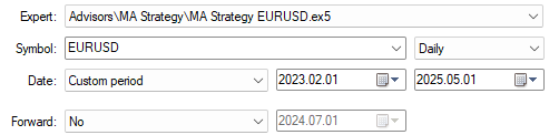
Figure 4: Our back test days are always outside the training period we showed the model.
Be sure to select "Random delay" for a realistic simulation of the unpredictable nature of real trading sessions.
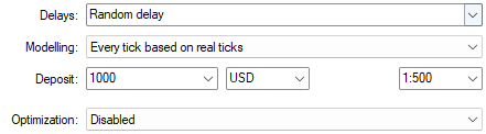
Figure 5: Select "Random delay" for the most robust back test settings available.
Our strategy produced the equity curve depicted in Figure 6. We are glad to see that we still managed to maintain a positive upward trend even when testing our model with data it has not seen before. It is possible that by training the model with a high-resolution picture of the market using the 40 columns we generated, our model is able to generalize better to conditions it has not been trained on.
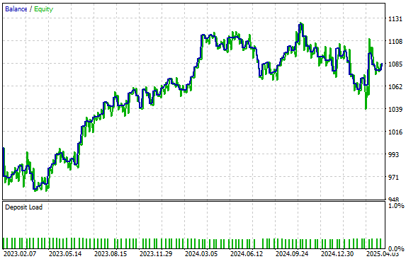
Figure 6: Visualizing the equity curve produced by our statistical model.
Lastly, we can always view a detailed summary of our strategy's performance. We can observe that 52.9% of the trades our strategy placed were profitable, and that our average profit is generally expected to be larger than our average loss. These are encouraging statistics and they demonstrate the virtue that can be uncovered by taking your time to craft detailed features into your datasets, although this can be a tedious process, it is always worth the additional effort when it pays off.
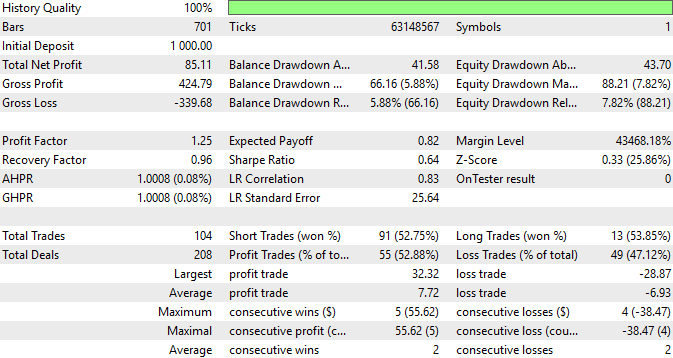
Figure 7: An in-depth summary of the performance attained by our trading application.
Conclusion
In conclusion, this article has provided the reader with numerous practical insights into how established strategies can be reimagined and infused with new abilities.
By leveraging well-known principles of data science, such as the ability for models to sometimes perform better in higher-dimensional spaces, we were able to consistently mitigate the lag in our moving average crossover strategies. This was achieved by handcrafting our own rich datasets, which allowed our model to gain a high-resolution understanding of the market. While these data science principles are well-studied, it is crucial to manage expectations.
It is important for the reader to note that inflating datasets into higher dimensions does not always guarantee better performance. Rather, readers should understand that it is always beneficial to investigate whether projecting datasets into higher dimensions can yield improvements. This approach offers no guarantees, but it is consistently worth exploring. The reader has also learned that the lag associated with technical indicators can be challenged and effectively addressed through critical thinking and creativity. The potential within the MetaTrader 5 terminal appears to be vast.
| File Name | File Description |
|---|---|
| EURUSD GBR MA D1.onnx | The ONNX model we built together using our high-dimensional column dataset. |
| Proof of Case Article.ipynb | The Jupyter Notebook we wrote together to demonstrate the virtue of projecting data to higher dimensions. |
| MA Strategy EURUSD.ex5 | A compiled version of the trading application we developed to take advantage of our hand-crafter dataset. |
| Fetch Data MA.mq5 | The MQL5 script we wrote to fetch our high-dimensional dataset and write it to CSV. |
Warning: All rights to these materials are reserved by MetaQuotes Ltd. Copying or reprinting of these materials in whole or in part is prohibited.
This article was written by a user of the site and reflects their personal views. MetaQuotes Ltd is not responsible for the accuracy of the information presented, nor for any consequences resulting from the use of the solutions, strategies or recommendations described.

- Free trading apps
- Over 8,000 signals for copying
- Economic news for exploring financial markets
You agree to website policy and terms of use