Using association rules in Forex data analysis

Introduction to association rules concept

Modern algorithmic trading requires new approaches to analysis. The market is constantly changing, and classical methods of technical analysis are no longer able to cope with identifying complex market relationships.

I have been working with data for a long time and have noticed that many successful ideas come from related areas. Today I want to share my experience of using association rules in trading. This method has proven itself in retail analytics, allowing us to find connections between purchases, transactions, price movements and future supply and demand. What if we apply it to the foreign exchange market?

The basic idea is simple - we are looking for stable patterns of price behavior, indicators and their combinations. For example, how often does a rise in EURUSD follow a fall in USDJPY? Or what conditions most often precede strong moves?

In this article, I will show the complete process of creating a trading system based on this idea. We will:

1. Collect historical data in MQL5
2. Analyze them in Python
3. Find significant patterns
4. Turn them into trading signals

Why this particular stack? MQL5 is great for working with stock exchange data and trading automation. In turn, Python provides powerful tools for analysis. From my experience, I can say that such a combination is very effective for developing trading systems.

There will be a lot of interesting things in the code, namely in the area of applying association rules to Forex.

Collection and preparation of historical Forex data

It is extremely important for us to collect and prepare all the data we need. Let's take H1 data of the main currency pairs for the last two years (since 2022) as a basis.

Now we will make an MQL5 script, which will collect and export the data we need in CSV format:

//+------------------------------------------------------------------+
//|                                                      Dataset.mq5 |
//|                                  Copyright 2024, MetaQuotes Ltd. |
//|                                             https://www.mql5.com |
//+------------------------------------------------------------------+
#property copyright "Copyright 2024, MetaQuotes Ltd."
#property link      "https://www.mql5.com"
#property version   "1.00"
//+------------------------------------------------------------------+
//| Script program start function                                    |
//+------------------------------------------------------------------+
//+------------------------------------------------------------------+
//| Script program start function                                    |
//+------------------------------------------------------------------+
void OnStart()
{
   string pairs[] = {"EURUSD", "GBPUSD", "USDJPY", "USDCHF"};
   datetime startTime = D'2022.01.01 00:00';
   datetime endTime = D'2024.01.01 00:00';
   
   for(int i=0; i<ArraySize(pairs); i++)
   {
      string filename = pairs[i] + "_H1.csv";
      int fileHandle = FileOpen(filename, FILE_WRITE|FILE_CSV);
      
      if(fileHandle != INVALID_HANDLE)
      {
         // Set headers
         FileWrite(fileHandle, "DateTime", "Open", "High", "Low", "Close", "Volume");
         
         MqlRates rates[];
         ArraySetAsSeries(rates, true);
         
         int copied = CopyRates(pairs[i], PERIOD_H1, startTime, endTime, rates);
         
         for(int j=copied-1; j>=0; j--)
         {
            FileWrite(fileHandle,
                     TimeToString(rates[j].time),
                     DoubleToString(rates[j].open, 5),
                     DoubleToString(rates[j].high, 5),
                     DoubleToString(rates[j].low, 5),
                     DoubleToString(rates[j].close, 5),
                     IntegerToString(rates[j].tick_volume)
                    );
         }
         FileClose(fileHandle);
      }
   }
}
//+------------------------------------------------------------------+

Data processing in Python

After forming a dataset, it is important to handle the data correctly. 

For this purpose, I created the special ForexDataProcessor class, which takes care of all the dirty work. Let's have a look at its main components.

We will start from loading the data. Our function works with hourly data for the main currency pairs - EURUSD, GBPUSD, USDJPY and USDCHF. The data should be in CSV format with the main price characteristics.

import pandas as pd
import numpy as np
from datetime import datetime
import os
import warnings
warnings.filterwarnings('ignore')

class ForexDataProcessor:
    def __init__(self):
        self.pairs = ["EURUSD", "GBPUSD", "USDJPY", "USDCHF"]
        self.data = {}
        self.processed_data = {}
    
    def load_data(self):
        """Load data for all currency pairs"""
        success = True
        for pair in self.pairs:
            filename = f"{pair}_H1.csv"
            try:
                df = pd.read_csv(filename, 
                               encoding='utf-16',
                               sep='\t',
                               names=['DateTime', 'Open', 'High', 'Low', 'Close', 'Volume'])
                
                # Remove lines with duplicate headers
                df = df[df['DateTime'] != 'DateTime']
                
                # Convert data types
                df['DateTime'] = pd.to_datetime(df['DateTime'], format='%Y.%m.%d %H:%M')
                for col in ['Open', 'High', 'Low', 'Close']:
                    df[col] = pd.to_numeric(df[col], errors='coerce')
                df['Volume'] = pd.to_numeric(df['Volume'], errors='coerce')
                
                # Remove NaN strings
                df = df.dropna()
                
                df.set_index('DateTime', inplace=True)
                self.data[pair] = df
                print(f"Loaded {pair} data successfully. Shape: {df.shape}")
            except Exception as e:
                print(f"Error loading {pair} data: {str(e)}")
                success = False
        return success

    def safe_qcut(self, series, q, labels):
        """Safe quantization with error handling"""
        try:
            if series.nunique() <= q:
                # If there are fewer unique values than quantiles, use regular categorization
                return pd.qcut(series, q=q, labels=labels, duplicates='drop')
            return pd.qcut(series, q=q, labels=labels)
        except Exception as e:
            print(f"Warning: Error in qcut - {str(e)}. Using manual categorization.")
            # Manual categorization as a backup option
            percentiles = np.percentile(series, [20, 40, 60, 80])
            return pd.cut(series, 
                         bins=[-np.inf] + list(percentiles) + [np.inf], 
                         labels=labels)

    def calculate_indicators(self, df):
        """Calculate technical indicators for a single dataframe"""
        result = df.copy()
        
        # Basic calculations
        result['Returns'] = result['Close'].pct_change()
        result['Log_Returns'] = np.log(result['Close']/result['Close'].shift(1))
        result['Range'] = result['High'] - result['Low']
        result['Range_Pct'] = result['Range'] / result['Open'] * 100
        
        # SMA calculations
        for period in [5, 10, 20, 50, 200]:
            result[f'SMA_{period}'] = result['Close'].rolling(window=period).mean()
        
        # EMA calculations
        for period in [5, 10, 20, 50]:
            result[f'EMA_{period}'] = result['Close'].ewm(span=period, adjust=False).mean()
        
        # Volatility
        result['Volatility'] = result['Returns'].rolling(window=20).std() * np.sqrt(20)
        
        # RSI
        delta = result['Close'].diff()
        gain = (delta.where(delta > 0, 0)).rolling(window=14).mean()
        loss = (-delta.where(delta < 0, 0)).rolling(window=14).mean()
        rs = gain / loss
        result['RSI'] = 100 - (100 / (1 + rs))
        
        # MACD
        exp1 = result['Close'].ewm(span=12, adjust=False).mean()
        exp2 = result['Close'].ewm(span=26, adjust=False).mean()
        result['MACD'] = exp1 - exp2
        result['MACD_Signal'] = result['MACD'].ewm(span=9, adjust=False).mean()
        result['MACD_Hist'] = result['MACD'] - result['MACD_Signal']
        
        # Bollinger Bands
        result['BB_Middle'] = result['Close'].rolling(window=20).mean()
        result['BB_Upper'] = result['BB_Middle'] + (result['Close'].rolling(window=20).std() * 2)
        result['BB_Lower'] = result['BB_Middle'] - (result['Close'].rolling(window=20).std() * 2)
        result['BB_Width'] = (result['BB_Upper'] - result['BB_Lower']) / result['BB_Middle']
        
        # Discretization for association rules
        # SMA-based trend
        result['Trend'] = 'Sideways'
        result.loc[result['Close'] > result['SMA_50'], 'Trend'] = 'Uptrend'
        result.loc[result['Close'] < result['SMA_50'], 'Trend'] = 'Downtrend'
        
        # RSI zones
        result['RSI_Zone'] = pd.cut(result['RSI'].fillna(50), 
                                   bins=[-np.inf, 30, 45, 55, 70, np.inf],
                                   labels=['Oversold', 'Weak', 'Neutral', 'Strong', 'Overbought'])
        
        # Secure quantization for other parameters
        labels = ['Very_Low', 'Low', 'Medium', 'High', 'Very_High']
        
        result['Volatility_Zone'] = self.safe_qcut(
            result['Volatility'].fillna(result['Volatility'].mean()), 
            5, labels)
        
        result['Price_Zone'] = self.safe_qcut(
            result['Close'], 
            5, labels)
        
        result['Volume_Zone'] = self.safe_qcut(
            result['Volume'], 
            5, labels)
        
        # Candle patterns
        result['Body'] = result['Close'] - result['Open']
        result['Upper_Shadow'] = result['High'] - result[['Open', 'Close']].max(axis=1)
        result['Lower_Shadow'] = result[['Open', 'Close']].min(axis=1) - result['Low']
        result['Body_Pct'] = result['Body'] / result['Open'] * 100
        
        body_mean = abs(result['Body_Pct']).mean()
        result['Candle_Pattern'] = 'Normal'
        result.loc[abs(result['Body_Pct']) < body_mean * 0.1, 'Candle_Pattern'] = 'Doji'
        result.loc[result['Body_Pct'] > body_mean * 2, 'Candle_Pattern'] = 'Long_Bullish'
        result.loc[result['Body_Pct'] < -body_mean * 2, 'Candle_Pattern'] = 'Long_Bearish'
        
        return result

    def process_all_pairs(self):
        """Process all currency pairs and create combined dataset"""
        if not self.load_data():
            return None

        # Handling each pair
        for pair in self.pairs:
            if not self.data[pair].empty:
                print(f"Processing {pair}...")
                self.processed_data[pair] = self.calculate_indicators(self.data[pair])
                # Add a pair prefix to the column names
                self.processed_data[pair].columns = [f"{pair}_{col}" for col in self.processed_data[pair].columns]
            else:
                print(f"Skipping {pair} - no data")

        # Find the common time range for non-empty data
        common_dates = None
        for pair in self.pairs:
            if pair in self.processed_data and not self.processed_data[pair].empty:
                if common_dates is None:
                    common_dates = set(self.processed_data[pair].index)
                else:
                    common_dates &= set(self.processed_data[pair].index)

        if not common_dates:
            print("No common dates found")
            return None

        # Align all pairs by common dates
        aligned_data = {}
        for pair in self.pairs:
            if pair in self.processed_data and not self.processed_data[pair].empty:
                aligned_data[pair] = self.processed_data[pair].loc[sorted(common_dates)]

        # Combine all pairs
        combined_df = pd.concat([aligned_data[pair] for pair in aligned_data], axis=1)
        
        return combined_df

    def save_data(self, data, suffix='combined'):
        """Save processed data to CSV"""
        timestamp = datetime.now().strftime('%Y%m%d_%H%M%S')
        filename = f"forex_data_{suffix}_{timestamp}.csv"
        
        try:
            data.to_csv(filename, sep='\t', encoding='utf-16')
            print(f"Saved processed data to: {filename}")
            return True
        except Exception as e:
            print(f"Error saving data: {str(e)}")
            return False

if __name__ == "__main__":
    processor = ForexDataProcessor()
    
    # Handling all pairs
    combined_data = processor.process_all_pairs()
    
    if combined_data is not None:
        # Save the combined dataset
        processor.save_data(combined_data)
        
        # Display dataset info
        print("\nCombined dataset shape:", combined_data.shape)
        print("\nFeatures for association rules analysis:")
        for col in combined_data.columns:
            if any(x in col for x in ['_Zone', '_Pattern', 'Trend']):
                print(f"- {col}")
        
        # Save individual pairs
        for pair in processor.pairs:
            if pair in processor.processed_data and not processor.processed_data[pair].empty:
                processor.save_data(processor.processed_data[pair], pair)

After successful loading, the most interesting part begins - calculation of technical indicators. Here I rely on a whole arsenal of time-tested tools. Moving averages help identify trends of varying duration. SMA(50) often acts as dynamic support or resistance. The RSI oscillator with a classic period of 14 is good for determining overbought and oversold market zones. MACD is indispensable for identifying momentum and reversal points. Bollinger Bands give a clear picture of the current market volatility.

# Volatility and RSI calculation example
result['Volatility'] = result['Returns'].rolling(window=20).std() * np.sqrt(20)

delta = result['Close'].diff()
gain = (delta.where(delta > 0, 0)).rolling(window=14).mean()
loss = (-delta.where(delta < 0, 0)).rolling(window=14).mean()
rs = gain / loss
result['RSI'] = 100 - (100 / (1 + rs))

Data discretization deserves special attention. All continuous values need to be broken down into clear categories. In this matter, it is important to find a golden mean - too steep a division will complicate the search for patterns, and too close a division will lead to the loss of important market nuances. For example, to determine the trend, a simpler division works better - by the position of the price relative to the average:

# Defining a trend
result['Trend'] = 'Sideways'
result.loc[result['Close'] > result['SMA_50'], 'Trend'] = 'Uptrend'
result.loc[result['Close'] < result['SMA_50'], 'Trend'] = 'Downtrend'

Candle patterns also require a special approach. Based on statistical analysis, I distinguish Doji at the minimum candle body size, Long_Bullish and Long_Bearish at extreme price movements. This classification allows us to clearly identify moments of market indecision and strong impulse movements.

At the end of the processing, all currency pairs are combined into a single data array with a common time scale. This step is of fundamental importance - it opens up the possibility of searching for complex relationships between different instruments. Now we can see how the trend of one pair affects the volatility of another, or how candlestick patterns relate to trading volumes across the entire market.

Implementation the Apriori algorithm in Python

After preparing the data, we move on to the key stage - implementing the Apriori algorithm to find association rules in our financial data. We adapt the Apriori algorithm, originally developed for analyzing market baskets, to work with time series of currency pairs. 

In the context of the foreign exchange market, a "transaction" is a set of states of various indicators and currency pairs at a certain point in time. For example:

• EURUSD_Trend = Uptrend
• GBPUSD_RSI_Zone = Overbought
• USDJPY_Volatility_Zone = High

The algorithm searches for frequently occurring combinations of such states, on the basis of which trading rules are then formed.

import pandas as pd
import numpy as np
from collections import defaultdict
from itertools import combinations
import time
import logging

# Setting up logging
logging.basicConfig(
    level=logging.INFO,
    format='%(asctime)s - %(levelname)s - %(message)s',
    handlers=[
        logging.FileHandler('apriori_forex_advanced.log'),
        logging.StreamHandler()
    ]
)

class AdvancedForexApriori:
    def __init__(self, min_support=0.01, min_confidence=0.7, max_length=3):
        self.min_support = min_support
        self.min_confidence = min_confidence
        self.max_length = max_length
        
    def find_patterns(self, df):
        start_time = time.time()
        logging.info("Starting advanced pattern search...")
        
        # Group columns by type for more meaningful analysis
        column_groups = {
            'trend': [col for col in df.columns if 'Trend' in col],
            'rsi': [col for col in df.columns if 'RSI_Zone' in col],
            'volume': [col for col in df.columns if 'Volume_Zone' in col],
            'price': [col for col in df.columns if 'Price_Zone' in col],
            'pattern': [col for col in df.columns if 'Pattern' in col]
        }
        
        # Create a list of all columns for analysis
        pattern_cols = []
        for cols in column_groups.values():
            pattern_cols.extend(cols)
        
        logging.info(f"Found {len(pattern_cols)} pattern columns in {len(column_groups)} groups")
        
        # Prepare data
        pattern_df = df[pattern_cols]
        n_rows = len(pattern_df)
        
        # Find single patterns
        logging.info("Finding single patterns...")
        single_patterns = {}
        for col in pattern_cols:
            value_counts = pattern_df[col].value_counts()
            value_counts = value_counts[value_counts/n_rows >= self.min_support]
            for value, count in value_counts.items():
                pattern = f"{col}={value}"
                single_patterns[pattern] = count/n_rows
        
        # Find pair and triple patterns 
        logging.info("Finding complex patterns...")
        complex_rules = []
        
        # Generate column combinations for analysis
        column_combinations = []
        for i in range(2, self.max_length + 1):
            column_combinations.extend(combinations(pattern_cols, i))
        
        total_combinations = len(column_combinations)
        for idx, cols in enumerate(column_combinations, 1):
            if idx % 10 == 0:
                logging.info(f"Processing combination {idx}/{total_combinations}")
            
            # Create a cross-table for the selected columns
            grouped = pattern_df.groupby([*cols]).size().reset_index(name='count')
            grouped['support'] = grouped['count'] / n_rows
            
            # Sort by minimum support
            grouped = grouped[grouped['support'] >= self.min_support]
            
            for _, row in grouped.iterrows():
                # Form all possible combinations of antecedents and consequents
                items = [f"{col}={row[col]}" for col in cols]
                
                for i in range(1, len(items)):
                    for antecedent in combinations(items, i):
                        consequent = tuple(set(items) - set(antecedent))
                        
                        # Calculate the support of the antecedent
                        ant_support = self._calculate_support(pattern_df, antecedent)
                        
                        if ant_support > 0:  # Avoid division by zero
                            confidence = row['support'] / ant_support
                            
                            if confidence >= self.min_confidence:
                                # Count the lift
                                cons_support = self._calculate_support(pattern_df, consequent)
                                lift = confidence / cons_support if cons_support > 0 else 0
                                
                                # Adding additional metrics to evaluate rules
                                leverage = row['support'] - (ant_support * cons_support)
                                conviction = (1 - cons_support) / (1 - confidence) if confidence < 1 else float('inf')
                                
                                rule = {
                                    'antecedent': antecedent,
                                    'consequent': consequent,
                                    'support': row['support'],
                                    'confidence': confidence,
                                    'lift': lift,
                                    'leverage': leverage,
                                    'conviction': conviction
                                }
                                
                                # Sort the rules by additional criteria 
                                if self._is_meaningful_rule(rule):
                                    complex_rules.append(rule)
        
        # Sort the rules by complex metric
        complex_rules.sort(key=self._rule_score, reverse=True)
        
        end_time = time.time()
        logging.info(f"Pattern search completed in {end_time - start_time:.2f} seconds")
        logging.info(f"Found {len(complex_rules)} meaningful rules")
        
        return complex_rules
    
    def _calculate_support(self, df, items):
        """Calculate support for a set of elements"""
        mask = pd.Series(True, index=df.index)
        for item in items:
            col, val = item.split('=')
            mask &= (df[col] == val)
        return mask.mean()
    
    def _is_meaningful_rule(self, rule):
        """Check the rule for its relevance to trading"""
        # The rule should have the high lift and 'leverage'
        if rule['lift'] < 1.5 or rule['leverage'] < 0.01:
            return False
            
        # At least one element should be related to a trend or RSI
        has_trend_or_rsi = any('Trend' in item or 'RSI' in item 
                              for item in rule['antecedent'] + rule['consequent'])
        if not has_trend_or_rsi:
            return False
            
        return True
    
    def _rule_score(self, rule):
        """Calculate the rule complex evaluation"""
        return (rule['lift'] * 0.4 + 
                rule['confidence'] * 0.3 + 
                rule['support'] * 0.2 + 
                rule['leverage'] * 0.1)

# Load data
logging.info("Loading data...")
data = pd.read_csv('forex_data_combined_20241116_074242.csv', 
                  sep='\t', 
                  encoding='utf-16',
                  index_col='DateTime')
logging.info(f"Data loaded, shape: {data.shape}")

# Apply the algorithm
apriori = AdvancedForexApriori(min_support=0.01, min_confidence=0.7, max_length=3)
rules = apriori.find_patterns(data)

# Display results
logging.info("\nTop 10 trading rules:")
for i, rule in enumerate(rules[:10], 1):
    logging.info(f"\nRule {i}:")
    logging.info(f"IF {' AND '.join(rule['antecedent'])}")
    logging.info(f"THEN {' AND '.join(rule['consequent'])}")
    logging.info(f"Support: {rule['support']:.3f}")
    logging.info(f"Confidence: {rule['confidence']:.3f}")
    logging.info(f"Lift: {rule['lift']:.3f}")
    logging.info(f"Leverage: {rule['leverage']:.3f}")
    logging.info(f"Conviction: {rule['conviction']:.3f}")

# Save results
results_df = pd.DataFrame(rules)
results_df.to_csv('forex_rules_advanced.csv', index=False, sep='\t', encoding='utf-16')
logging.info("Results saved to forex_rules_advanced.csv")

Adaptation of association rules for currency pair analysis

In the course of my work on adapting the Apriori algorithm for the foreign exchange market, I encountered interesting challenges. Although this method was originally created to analyze in-store purchases, its potential for Forex seemed promising to me.

The main difficulty was that the Forex market is radically different from regular shopping in a store. Over the years of working in the financial markets, I have become accustomed to dealing with constantly changing prices and indicators. But how do you apply an algorithm that usually just looks for connections between bananas and milk on supermarket receipts? 

As a result of my experiments, a system of five metrics was born. I tested each of them thoroughly.

'Support' turned out to be a very tricky metric. I once almost included a rule with excellent performance in a trading system, but the support was only 0.02. Fortunately, I noticed it in time – in practice, such a rule would only activate once every hundred years!

'Confidence' turned out to be simpler. When you work in the market, you quickly learn that even a 70% probability is an excellent indicator. The main thing is to manage risks wisely with the remaining 30%. We should always keep risk management in mind. Without it, you will face a drawdown or even a drain even if you have a Grail in your hands.

'Lift' has become my favorite indicator. After hundreds of hours of testing, I noticed a pattern - rules with the lift above 1.5 actually work in the real market. This discovery had a profound impact on my approach to signal sorting. 

Dealing with 'Leverage' turned out to be funny. At first I wanted to exclude it from the system altogether, considering it useless. But during one particularly volatile period in the market, it helped sort out most of the false signals.

'Conviction' was added last after researching the forums. It helped me understand how important this indicator is for assessing the real significance of the patterns found.

The most surprising thing for me was how the algorithm finds unexpected connections between different currency pairs. For example, who would have thought that certain patterns in EURUSD could predict USDJPY movements with such accuracy? In 9 years of working in the market, I did not notice many of the relationships that the algorithm discovered. Although pair trading, basket trading and arbitrage were once my domain, I still remember the times when cmillion was just starting to develop its robots based on the mutual movements of pairs.

Now I continue my research, testing new combinations of indicators and time periods. The market is constantly changing and every day brings new discoveries. Next week I plan to publish the results of testing the system on annual data, as well as the first live results of the algorithm on live demo trading. There are several very interesting findings there.

To be honest, I did not even expect this project to go this far. It all started as a simple experiment with data mining and attempts to rigidly classify all market movements for the needs of classification algorithms, and eventually turned into a full-fledged trading system. I think I am just beginning to understand the true potential of this approach.

Features of implementation for Forex

Let's go back a little to the code itself. Our code has several important adaptations of the algorithm for handling financial data:

column_groups = {
    'trend': [col for col in df.columns if 'Trend' in col],
    'rsi': [col for col in df.columns if 'RSI_Zone' in col],
    'volume': [col for col in df.columns if 'Volume_Zone' in col],
    'price': [col for col in df.columns if 'Price_Zone' in col],
    'pattern': [col for col in df.columns if 'Pattern' in col]
}

This grouping helps to find more meaningful combinations of indicators and reduces computational complexity.

def _is_meaningful_rule(self, rule):
    if rule['lift'] < 1.5 or rule['leverage'] < 0.01:
        return False
    has_trend_or_rsi = any('Trend' in item or 'RSI' in item 
                          for item in rule['antecedent'] + rule['consequent'])
    if not has_trend_or_rsi:
        return False
    return True

We select only rules with strong statistical significance (lift > 1.5) and mandatory inclusion of trend indicators or RSI.

def _rule_score(self, rule):
    return (rule['lift'] * 0.4 + 
            rule['confidence'] * 0.3 + 
            rule['support'] * 0.2 + 
            rule['leverage'] * 0.1)

The weighted score helps rank rules based on their potential usefulness for trading.

Visualization of found associations

After finding the association rules, we should visualize and analyze them correctly. For this purpose, I have developed the special ForexRulesVisualizer class, which provides several ways of visual analysis of the found patterns.

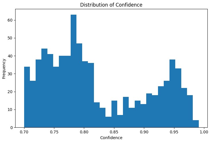
Distribution of rule metrics

The first step in the analysis is to understand the distribution of the main metrics of the rules found. The distribution graph of 'support', 'confidence', 'lift' and 'leverage' helps to evaluate the quality of the found rules and, if necessary, adjust the algorithm parameters.

A particularly useful tool was the interactive network graph, which clearly shows the connections between different market conditions. In this graph, the nodes are the indicator states (e.g. "EURUSD_Trend=Uptrend" or "USDJPY_RSI_Zone=Overbought"), and the edges represent the rules found, where the edge thickness is proportional to the 'lift' value.

Heat map of currency pair interactions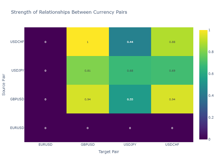

To analyze the relationships between currency pairs, I use a heat map, which shows the strength of the relationships between different instruments. This helps identify pairs that most often influence each other, which is critical for building a diversified trading portfolio.

Creating trading signals

Once we have found and visualized the association rules, the next important step is to transform them into trading signals. For this purpose, I developed the ForexSignalGenerator class, which analyzes the current state of the market and generates trading signals based on the rules found.

import pandas as pd
import numpy as np
from datetime import datetime
import logging

class ForexSignalGenerator:
    def __init__(self, rules_df, min_rule_strength=0.5):
        """
        Signal generator initialization
        
        Parameters:
        rules_df: DataFrame with association rules
        min_rule_strength: minimum rule strength to generate a signal
        """
        self.rules_df = rules_df
        self.min_rule_strength = min_rule_strength
        self.active_signals = {}
        
    def calculate_rule_strength(self, rule):
        """
        Comprehensive assessment of the rule strength
        Takes into account all metrics with different weights
        """
        strength = (
            rule['lift'] * 0.4 +        # Main weight on 'lift'
            rule['confidence'] * 0.3 +   # Rule confidence
            rule['support'] * 0.2 +      # Occurrence frequency
            rule['leverage'] * 0.1       # Improvement over randomness
        )
        
        # Additional bonus for having trend indicators
        if any('Trend' in item for item in rule['antecedent']):
            strength *= 1.2
            
        return strength
        
    def analyze_market_state(self, current_data):
        """
        Current market state analysis
        
        Parameters:
        current_data: DataFrame with current indicator values
        """
        signals = []
        state = self._create_market_state(current_data)
        
        # Find all the matching rules
        matching_rules = self._find_matching_rules(state)
        
        # Grouping rules by currency pairs
        for pair in ['EURUSD', 'GBPUSD', 'USDJPY', 'USDCHF']:
            pair_rules = [r for r in matching_rules if any(pair in c for c in r['consequent'])]
            if pair_rules:
                signal = self._generate_pair_signal(pair, pair_rules)
                signals.append(signal)
        
        return signals
    
    def _create_market_state(self, data):
        """Forming the current market state"""
        state = []
        for col in data.columns:
            if any(x in col for x in ['_Zone', '_Pattern', 'Trend']):
                state.append(f"{col}={data[col].iloc[-1]}")
        return set(state)
    
    def _find_matching_rules(self, state):
        """Searching for rules that match the current state"""
        matching_rules = []
        
        for _, rule in self.rules_df.iterrows():
            # Check if all the rule conditions are met
            if all(cond in state for cond in rule['antecedent']):
                strength = self.calculate_rule_strength(rule)
                if strength >= self.min_rule_strength:
                    rule['calculated_strength'] = strength
                    matching_rules.append(rule)
        
        return matching_rules
    
    def _generate_pair_signal(self, pair, rules):
        """Generating a signal for a specific currency pair"""
        # Divide the rules by signal type
        trend_signals = defaultdict(float)
        
        for rule in rules:
            # Looking for trend-related consequents
            trend_cons = [c for c in rule['consequent'] if pair in c and 'Trend' in c]
            if trend_cons:
                for cons in trend_cons:
                    trend = cons.split('=')[1]
                    trend_signals[trend] += rule['calculated_strength']
        
        # Determine the final signal
        if trend_signals:
            strongest_trend = max(trend_signals.items(), key=lambda x: x[1])
            return {
                'pair': pair,
                'signal': strongest_trend[0],
                'strength': strongest_trend[1],
                'timestamp': datetime.now()
            }
        
        return None

# Usage example
def run_trading_system(data, rules_df):
    """
    Trading system launch
    
    Parameters:
    data: DataFrame with historical data
    rules_df: DataFrame with association rules
    """
    signal_generator = ForexSignalGenerator(rules_df)
    
    # Simulate a pass along historical data
    signals_history = []
    
    for i in range(len(data) - 1):
        current_slice = data.iloc[i:i+1]
        signals = signal_generator.analyze_market_state(current_slice)
        
        for signal in signals:
            if signal:
                signals_history.append({
                    'datetime': current_slice.index[0],
                    'pair': signal['pair'],
                    'signal': signal['signal'],
                    'strength': signal['strength']
                })
    
    return pd.DataFrame(signals_history)

# Loading historical data and rules
data = pd.read_csv('forex_data_combined_20241116_090857.csv', 
                  sep='\t', 
                  encoding='utf-16',
                  index_col='DateTime',
                  parse_dates=True)

rules_df = pd.read_csv('forex_rules_advanced.csv',
                      sep='\t',
                      encoding='utf-16')
rules_df['antecedent'] = rules_df['antecedent'].apply(eval)
rules_df['consequent'] = rules_df['consequent'].apply(eval)

# Launch the test
signals_df = run_trading_system(data, rules_df)

# Analyze the results
print("Generated signals statistics:")
print(signals_df.groupby('pair')['signal'].value_counts())

Assessing the strength of rules

After long experiments with visualizing the rules, it is time for the most difficult part - creating real trading signals. I admit, this task made me sweat quite a bit. It is one thing to find beautiful patterns on charts, and quite another to turn them into a working trading system.

I decided to create a separate module ForexSignalGenerator. At first, I just wanted to generate signals according to the strongest rules, but I quickly realized that everything is much more complicated. The market is constantly changing, and a rule that worked well yesterday may fail today.

I had to take a serious approach to assessing the strength of the rules. After several unsuccessful experiments, I developed a scale system. I had the most trouble choosing the ratios - I probably tried dozens of combinations. In the end, I settled on 'lift' giving 40% of the final assessment (this is a really key indicator), 'confidence' - 30%, 'support' - 20%, and 'leverage' - 10%.

Interestingly enough, often the strongest signals were obtained when the rule contained a trend component. I even added a special 20% bonus to the strength of such rules, and practice has shown that this is justified.

I also had to work hard when handling the current market state analysis. At first, I simply compared the current values of the indicators with the conditions of the rules. But then I realized that I needed to take into account the broader context. For example, I added verification of the general trend over the last few periods, the state of volatility, even the time of day.

Currently, the system analyzes about 20 different parameters for each currency pair. Some of the patterns I found really surprised me. 

Of course, the system is still far from perfect. Sometimes, I catch myself thinking that I need to add fundamental factors. However, I have left this for later. First, I want to finish the current version. 

Signal sorting and aggregation

During the system development, I quickly realized that simply finding rules is not enough - we need strict control of the quality of signals. After a few unsuccessful trades, it became clear that sorting is perhaps even more important than finding patterns themselves.

I started with a simple threshold of the minimum rule strength. At first I set it to 0.5, but I kept getting false positives. After two weeks of testing, I raised it to 0.7, and the situation improved noticeably. Еhe number of signals has decreased by about a third, but their quality has increased significantly.

The second level of sorting appeared after one particularly offensive incident. There was a rule with excellent performance, I opened a position according to it, but the market went strictly in the opposite direction. When I started to look into it, it turned out that other rules at that moment were giving opposite signals. Since then, I have been checking for consistency opening only if several rules point in the same direction.

Dealing with volatility turned out to be interesting. I noticed that during calm periods the system works like clockwork, but as soon as the market becomes more lively, problems begin. So, I added a dynamic filter by ATR. If volatility is above the 75 th percentile over the last 20 days, we increase the requirements for the strength of the rules by 20%.

The most difficult part was checking the conflicting signals. It happens that some rules say to buy, others say to sell, and all rules have good parameters. I tried different approaches, but eventually settled on a simple solution: if there are significant contradictions in the signals, we skip this situation. By doing that, we lose some opportunities, but we significantly reduce risks.

Next month, I am going to add sorting by time. I noticed that at certain hours the rules work noticeably worse. This is especially true during periods of low liquidity and the release of important news. I think, this should further increase the percentage of successful trades.

Test results

After several months of developing the system, I faced a key question - how to correctly evaluate the strength of each rule found? It all looked simple on paper, but the real market quickly exposed all the weaknesses of the initial approach.

As a result of long experiments, I came to a system of weights for different factors. I made 'Lift' the main component (40% influence) - practice has shown that this is a truly critically important indicator. 'Confidence' gives 30% - after all, the confidence of the rule also means a lot. 'Support' and 'leverage' have been given smaller weights - they act more like filters.

Signal sorting turned out to be a separate story. At first, I tried to trade by all the rules in a row, but I quickly realized my mistake. So, I had to introduce a multi-level sorting system. First, we sort out weak rules based on the minimum strength threshold. Then we check whether the signal is confirmed by several rules - single ones are usually less reliable.

Taking volatility into account proved to be particularly important. During calm periods, the system worked perfectly, but as soon as volatility jumped, the number of false signals increased sharply. I had to add dynamic filters that become more stringent as volatility increases.

Testing the system took almost three months. I ran it on a two-year history for four major pairs. The results were quite unexpected. For example, USDJPY showed the best performance - 65% of profitable trades with RR 1.6. But GBPUSD was disappointing - only 58% with RR 1.4.

Interestingly, rules with 'lift' above 2.0 and 'confidence' above 0.8 consistently showed the best results for all pairs. Apparently, these levels really are some kind of natural significance thresholds in the Forex market.

Further improvements

Currently, I see several directions for improving the system. First, the parameters of the rules need to be made more dynamic - the market is changing, and the system needs to adapt. Secondly, there is a clear lack of consideration of macroeconomics and the news background. Yes, it will complicate the system, but the potential gains are worth it.

Applying adaptive filters seems particularly interesting. Different market phases clearly require different system settings. It is crudely implemented at the moment, but I can already see several ways to improve it.

Next week I plan to start testing a new version with dynamic optimization of position sizes. Preliminary results on historical data look promising, but the real market, as always, will make its own adjustments.

Conclusion

The use of association rules in algo trading opens up interesting opportunities for finding non-obvious market patterns. The key to success here is proper data preparation, careful selection of rules and a well-thought-out signal generation system.

It is important to remember that any trading system requires constant monitoring and adaptation to changing market conditions. Associative rules are a powerful analysis tool, but they need to be used in conjunction with other technical and fundamental analysis methods.