
Non-linear regression models on the stock exchange

Introduction
Yesterday I was once again sitting over the reports of my regression-based trading system. Wet snow was falling outside the window, the coffee was getting cold in the mug, but I still could not get rid of the obsessive thought. You know, I have long been irritated by these endless RSI, Stochastic, MACD and other indicators. How can we try to fit a living and dynamic market into these primitive equations? Every time I see another YouTube Grail proponent with his "sacred" set of indicators, I just want to ask - man, do you really believe that these calculators from the seventies can catch the complex dynamics of the modern market?
I have spent the last three years trying to create something that actually works. I have tried many things - from the simplest regressions to sophisticated neural networks. And you know what? I managed to achieve results in classification, but not yet in regression.
There was the same story every time - in history everything works like clockwork, but when I release it onto the real market, I face losses. I remember how excited I was about my first convolutional network. R2 at 1.00% on training. This was followed by two weeks of trading and minus 30% of the deposit. Classic overfitting at its finest. I kept enabling forward visualization watching how the regression-based forecast moves further and further away from the real prices, overtime...
But I am a stubborn person. After another loss, I decided to dig deeper and started sifting through scientific articles. And do you know what I dug up in the dusty archives? It turns out that old Mandelbrot was already harping on about the fractal nature of markets. And we are all trying to trade with linear models! It is like trying to measure the length of a coastline with a ruler - the more accurately you measure, the longer it gets.
At some point it dawned on me: what if I try to cross classical technical analysis with non-linear dynamics? Not these crude indicators, but something more serious - differential equations, adaptive ratios. It sounds complicated, but in essence it is simply an attempt to learn to speak the market in its language.
In short, I took Python, hooked up the machine learning libraries, and started experimenting. I decided right away - no academic bells and whistles, just what can really be used. No supercomputers - just a regular Acer laptop, super-powerful VPS and MetaTrader 5 terminal. From all this, the model that I want to tell you about was born.
No, it is not a Grail. Grails do not exist, I realized that a long time ago. I am just sharing my experience on applying modern mathematics to real trading. No unnecessary hype, but also no primitivism of "trend indicators". The result was something in between: smart enough to work, but not so complex that it would fall apart when meeting the first black swan event.
Mathematical model
I remember how I came up with this equation. I have been working on this code since 2022, but not constantly: in terms of approaches, I would say - there are many developments, so you periodically (a little chaotically) go through them and bring one after another to the result. I remember running charts, trying to catch patterns in EURUSD. And you know what caught my eye? The market seems to breathe - sometimes it flows smoothly along the trend, sometimes it suddenly jerks sharply, sometimes it enters into some kind of magical rhythm. How to describe this mathematically? How to capture this living dynamics in equations?
Afterwards, I sketched out the first version of the equation. Here it is, in all its glory:

And here it is in the code:
def equation(self, x_prev, coeffs):
    x_t1, x_t2 = x_prev[0], x_prev[1]
    return (coeffs[0] * x_t1 +          # trend
            coeffs[1] * x_t1**2 +       # acceleration
            coeffs[2] * x_t2 +          # market memory
            coeffs[3] * x_t2**2 +       # inertia
            coeffs[4] * (x_t1 - x_t2) + # impulse
            coeffs[5] * np.sin(x_t1) +  # market rhythm
            coeffs[6])                   # basic level
Look how everything is twisted. The first two terms are an attempt to catch the current market movement. Do you know how a car accelerates? First smoothly, then faster and faster. That is why there is both a linear and a quadratic term here. When the price moves calmly, the linear part works. But as soon as the market accelerates, the quadratic term picks up the movement.
Now comes the most interesting part. The third and fourth terms look a little deeper into the past. It is like a market memory. Do you recall the Dow Theory about the market remembering its levels? It is the same here. And again it features quadratic acceleration - to catch sharp turns.
Now the momentum component. We simply subtract the previous price from the current one. It would seem primitive. But it works cool on trend movements! When the market gets into a frenzy and pushes in one direction, this term becomes the main driving force of the forecast.
Sine was added almost by accident. I was looking at the charts and noticed some kind of periodicity. Especially on H1. Moves and calm periods followed one another... It looks like a sine wave, doesn't it? I put the sine wave into the equation, and the model seemed to see the light and began to catch these rhythms.
The last ratio is a kind of safety net, a basic level. This term does not allow the model to greatly surprise the market with its forecasts.
I tried a bunch of other options. I shoved exponents, logarithms, and all sorts of fancy trigonometric functions there. There is little point, but the model turns into a monster. You know, as Occam said: do not multiply entities beyond what is necessary. The current version turned out to be just like that - simple and working.
Of course, all these ratios need to be selected somehow. This is where the good old Nelder-Mead method comes to the rescue. But that is a completely different story I am going to reveal in the next part. Believe me, there is a lot to talk about - the mistakes I made during optimization alone would be enough for a separate article.
Linear componentsLet's start with the linear part. Do you know what the main thing is? The model looks at the two previous price values, but in different ways. The first ratio usually comes out to be around 0.3-0.4 - this is an instant reaction to the last change. But the second one is more interesting, it often approaches 0.7, which indicates a stronger influence of the penultimate price. Funny, huh? The market seems to be relying on slightly older levels, not trusting the latest fluctuations.
Quadratic componentsAn interesting story happened with the quadratic terms. Initially, I added them simply to account for non-linearity, but then I noticed something surprising. In a calm market, their contribution is negligible - the ratios fluctuate around 0.01-0.02. But as soon as a strong movement begins, these members seem to wake up. This is especially clear on the daily EURUSD charts - when the trend gains strength, the quadratic terms begin to dominate, allowing the model to "accelerate" along with the price.
Momentum componentThe momentum component turned out to be a real discovery. It would seem like a trivial price difference, but it reflects the market mood with sharp accuracy! During calm periods, its ratio remains around 0.2-0.3, but before strong movements it often jumps to 0.5. This became for me a kind of indicator of an impending breakthrough - when the optimizer starts to raise the momentum weight, expect movement.
Cyclic componentThe cyclic component required some tinkering. At first, I tried different periods of the sine wave, but then I realized that the market itself sets the rhythm. It is sufficient to let the model adjust the amplitude via the ratio, and the frequency is obtained naturally from the prices themselves. It is funny to watch how this ratio changes between the European and American sessions - as if the market really breathes at a different rhythm.
Finally, the free term. Its role turned out to be much more important than I initially thought. During periods of high volatility, it acts as an anchor, preventing forecasts from flying off into space. And in calm periods it helps to more accurately take into account the general price level. Quite often, its value correlates with the strength of the trend - the stronger the trend, the closer the free term is to zero.
Do you know what's most interesting? Every time I tried to complicate the model - add new terms, use more complex functions, etc., the results only got worse. It was as if the market was saying: "Boy, don't be smart, you've already caught the main thing". The current version of the equation is truly a happy medium between complexity and efficiency. There are seven ratios - no more and no less, each with its own clear role in the overall forecasting mechanism.
By the way, the optimization of these ratios is a fascinating story of its own. When you start to observe how the Nelder-Mead method searches for optimal values, you involuntarily recall chaos theory. But we will talk about this in the next part - there is something to see there, believe me.
Model optimization using the Nelder-Mead algorithm
Here we will consider the most interesting thing – how to make our model work on real data. After months of experimenting with optimization, dozens of sleepless nights and liters of coffee, I finally found a working approach.
It all started as usual - with gradient descent. A classic of the genre, the first thing that comes to any data scientist's mind. I spent three days on implementation, another week on debugging... So what were the results? The model categorically refused to converge. It would either fly off into infinity or get stuck in local minima. The gradients jumped like crazy.
Then there was a week with genetic algorithms. The idea is seemingly elegant - let evolution find the best ratios. I implemented it, launched it... just to be stunned by the running time. The computer hummed all night to handle one week of historical data. The results were so unstable that it was like reading tea leaves.
And then I came across the Nelder-Mead method. The good old simplex method, developed back in 1965. No derivatives, no higher mathematics - just smart probing of the solution space. I launched it and could not believe my eyes. The algorithm seemed to dance with the market, smoothly approaching optimal values.
Here is the basic loss function. It is as simple as an axe, but works flawlessly:
def loss_function(self, coeffs, X_train, y_train):
    y_pred = np.array([self.equation(x, coeffs) for x in X_train])
    mse = np.mean((y_pred - y_train)**2)
    r2 = r2_score(y_train, y_pred)

    # Save progress for analysis
    self.optimization_progress.append({
        'mse': mse,
        'r2': r2,
        'coeffs': coeffs.copy()
    })
    return mse
At first, I tried to complicate the loss function, adding penalties for large ratios, as well as shoving MAPE and other metrics into it. A classic developer mistake is that if something works, it must be improved until it becomes completely inoperable. In the end, I went back to simple MSE, and you know what? It turns out that simplicity really is a sign of genius.
It is a special thrill to watch the optimization in real time. First iterations - ratios are jumping like crazy, MSE is jumping, R² is close to zero. Then the most interesting part begins - the algorithm finds the right direction, and the metrics gradually improve. By the hundredth iteration, it is already clear whether there will be any benefit or not, and by the three hundredth, the system usually reaches a stable level.
By the way, let me say a few words about metrics. Our R² is usually over 0.996, which means that the model explains more than 99.6% of the price variation. The MSE is around 0.0000007 - in other words, the forecast error rarely exceeds seven tenths of a pip. As for MAPE... MAPE is generally pleasing - often less than 0.1%. It is clear that this is all based on historical data, but even on the forward test the results are not much worse.
But the most important thing is not even the numbers. The main thing is stability of results. You can run the optimization ten times in a row, and each time you will get very close ratio values. This is worth a lot, especially considering my struggles with other optimization methods.
You know what else is cool? By observing the optimization, you can understand a lot about the market itself. For example, when the algorithm constantly tries to increase the weight of the momentum component, it means that a strong movement is brewing in the market. Or when it starts playing with the cyclical component - expect a period of increased volatility.
In the next section, I will tell you how all this mathematical structure turns into a real trading system. Believe me, there is also something to think about there - the pitfalls regarding MetaTrader 5 alone are enough for a separate article.
Training process features
Preparing data for training was a separate story. I remember how in the first version of the system I happily fed the entire dataset to sklearn.train_test_split... And only later, looking at the suspiciously good results, I realized that future data is leaking into past!
Do you see what the problem is? You cannot treat financial data like a regular Kaggle spreadsheet. Here, each data point is a moment in time, and mixing them is like trying to predict yesterday's weather based on tomorrow's. As a result, this simple but efficient code was born:
def prepare_training_data(prices, train_ratio=0.67):
    # Cut off a piece for training
    n_train = int(len(prices) * train_ratio)

    # Forming prediction windows
    X = np.array([[prices[i], prices[i-1]] for i in range(2, len(prices)-1)])
    y = prices[3:]

    # Fair time sharing
    X_train, y_train = X[:n_train], y[:n_train]
    X_test, y_test = X[n_train:], y[n_train:]

    return X_train, y_train, X_test, y_test
It would seem to be a simple code. But behind this simplicity there is a lot of hard knocks. At first, I experimented with different window sizes. I thought the more historical points, the better the forecast. I was wrong! It turned out that the two previous values were quite sufficient. The market does not like to remember the past for long, you know.
The size of the training sample is a separate story. I tried different options – 50/50, 80/20, even 90/10. In the end, I settled on the golden ratio - approximately 67% of the training data. Why? It just works the best! Apparently old Fibonacci knew something about the nature of markets...
It is fun to watch the model training from different pieces of data. When taking a calm period, the ratios are selected smoothly and the metrics improve gradually. And if the training sample includes something like Brexit or a speech by the head of the Federal Reserve, all the hell goes loose: the ratios jump, the optimizer freaks out, and the error graphs draw a roller coaster.
By the way, let me say a few words about metrics again. I noticed that if R² on the training sample is higher than 0.98, it is almost certain that there was some kind of screw-up with the data. The real market simply cannot be that predictable. It is like that story about the too-good student - either he cheats or he is a genius. In our case, it is usually the former.
Another important point is data preprocessing. At first, I tried to normalize prices, scale, remove outliers... In general, I did everything that is taught in machine learning courses. But gradually I came to the conclusion that the less you touch the raw data, the better. The market will normalize itself, you just have to prepare everything correctly.
Now the training has been streamlined to the point of automatism. Once a week we load fresh data, run training, and compare metrics with historical values. If everything is within normal limits, update the ratios in the real-action system. If something is suspicious, dig deeper. Fortunately, experience already allows us to understand where to look for the problem.
Optimizing ratios
def fit(self, prices):
    # Prepare data for training
    X_train, y_train = self.prepare_training_data(prices)

    # I found these initial values by trial and error
    initial_coeffs = np.array([0.5, 0.1, 0.3, 0.1, 0.2, 0.1, 0.0])

    result = minimize(
        self.loss_function,
        initial_coeffs,
        args=(X_train, y_train),
        method='Nelder-Mead',
        options={
            'maxiter': 1000,  # More iterations does not improve the result
            'xatol': 1e-8,   # Accuracy by ratios
            'fatol': 1e-8    # Accuracy by loss function
        }
    )

    self.coefficients = result.x
    return result
Do you know what turned out to be the most difficult thing? Get those damn initial odds right. At first I tried to use random values - I got such a spread of results that I was ready to give up. Then I tried starting with ones - the optimizer flew off into space somewhere during the first iterations. It did not work with zeros either since it got stuck in local minima.
The first ratio 0.5 is the weight of the linear component. If it is less, the model loses its trend, if it is more, it starts to rely too much on the last price. For the quadratic terms, 0.1 turned out to be a perfect start - enough to catch non-linearity, but not so much that the model started to go crazy on sudden movements. The value of 0.2 for momentum was gained empirically; it is just that at this value the system showed the most stable results.
During the optimization, Nelder-Mead constructs a simplex in a seven-dimensional ratio space. It is like a game of hot and cold, only in seven dimensions at once. It is important to prevent process divergence, which is why there are such strict requirements for accuracy (1e-8). If it is less, we get unstable results, if it is more, optimization starts to get stuck in local minima.
A thousand iterations may seem excessive, but in practice the optimizer usually converges in 300-400 steps. It is just that sometimes, especially during periods of high volatility, he needs more time to find the optimal solution. And extra iterations do not really affect performance - the whole process usually takes less than a minute on modern hardware.
By the way, it was during the process of debugging this code that the idea was born to add visualization of the optimization process. When you see the odds changing in real time, it is much easier to understand what is going on with the model and where it might go.
Quality metrics and their interpretation
Assessing the quality of a predictive model is a separate story, full of non-obvious nuances. Over the years of working with algorithmic trading, I have suffered with metrics enough to write a separate book about it. But I will tell you about the main thing.
Here are the results:

Let's start with R-squared. The first time I saw values above 0.9 on EURUSD, I could not believe my eyes. I checked the code ten times to make sure there was no data leakage or calculation errors. There was none - the model does explain more than 90% of the price variance. However, later I realized that this is a double-edged sword. Too high R² (greater than 0.95) usually indicates overfitting. The market simply cannot be that predictable.
MSE is our workhorse. Here is a typical assessment code:
def evaluate_model(self, y_true, y_pred):
    results = {
        'R²': r2_score(y_true, y_pred),
        'MSE': mean_squared_error(y_true, y_pred),
        'MAPE': mean_absolute_percentage_error(y_true, y_pred) * 100
    }

    # Additional statistics that often save the day
    errors = y_pred - y_true
    results['max_error'] = np.max(np.abs(errors))
    results['error_std'] = np.std(errors)

    # Look separately at error distribution "tails"
    results['error_quantiles'] = np.percentile(np.abs(errors), [50, 90, 95, 99])

    return results
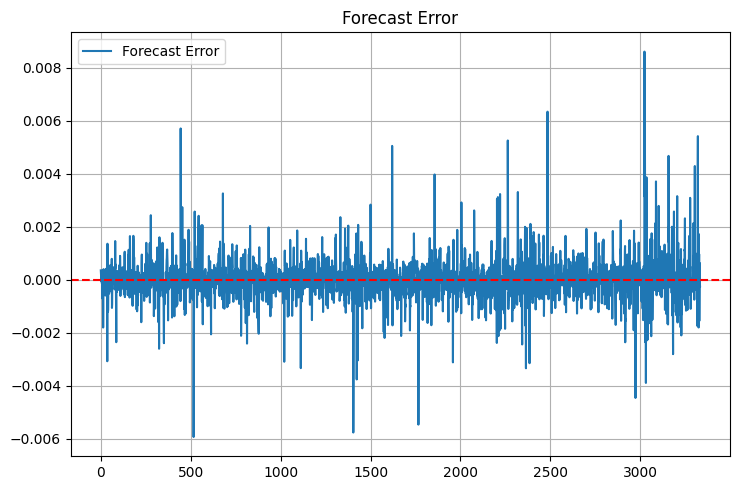
Please note the additional statistics. I added max_error and error_std after one unpleasant incident - the model showed excellent MSE, but sometimes it gave such outliers in forecasts that I could immediately close the deposit without even trying. Now the first thing I look at is the "tails" of the error distribution. However, the tails still exist:
MAPE is like home for traders. If you tell them about R-squared, their eyes become glassy, but if you say "the model is wrong by 0.05% on average", they immediately understand. There is a catch though - MAPE can be deceptively low during small price movements and skyrocket during sharp movements.
But the most important thing I understood is that no metrics based on historical data guarantee success in real life. That is why I now have a whole system of checks:
def validate_model_performance(self):
    # Check metrics on different timeframes
    timeframes = ['H1', 'H4', 'D1']
    for tf in timeframes:
        metrics = self.evaluate_on_timeframe(tf)
        if not self._check_metrics_thresholds(metrics):
            return False

    # Look at behavior at important historical events
    stress_periods = self.get_stress_periods()
    stress_metrics = self.evaluate_on_periods(stress_periods)
    if not self._check_stress_performance(stress_metrics):
        return False

    # Check the stability of forecasts
    stability = self.check_prediction_stability()
    if stability < self.min_stability_threshold:
        return False

    return True
The model should pass all these tests before I put it into real trading. And even after that, for the first two weeks I trade with a minimum volume - I check how it behaves on the live market.
People often ask, what metric values are considered good. According to my experience, R² higher than 0.9 is excellent, MSE less than 0.00001 is acceptable, while MAPE up to 0.05% is splendid. However! It is more important to look at the stability of these indicators over time. It is better to have a model with slightly worse but stable metrics than a super-accurate but unstable system.
Technical implementation
Do you know what the hardest thing is in developing trading systems? Not mathematics, not algorithms, but reliability of operation. It is one thing to write a beautiful equation, and quite another to make it work 24/7 with real money. After several painful screw-ups on a real account, I realized: architecture should not just be good, it should be impeccable.
This is how I arranged the system core:
class PriceEquationModel:
    def __init__(self):
        # Model status
        self.coefficients = None
        self.training_scores = []
        self.optimization_progress = []

        # Initializing the connection
        self._setup_logging()
        self._init_mt5()

    def _init_mt5(self):
        """Initializing connection to MT5"""
        try:
            if not mt5.initialize():
                raise ConnectionError(
                    "Unable to connect to MetaTrader 5. "
                    "Make sure the terminal is running"
                )
            self.log.info("MT5 connection established")
        except Exception as e:
            self.log.critical(f"Critical initialization error: {str(e)}")
            raise
Every string here is the result of some sad experience. For example, a separate method for initializing MetaTrader 5 appeared after I got a deadlock when trying to reconnect. And I added logging when the system silently crashed in the middle of the night, and in the morning I had to guess what happened.
Error handling is a whole other story.
def _safe_mt5_call(self, func, *args, retries=3, delay=5):
    """Secure MT5 function call with automatic recovery"""
    for attempt in range(retries):
        try:
            result = func(*args)
            if result is not None:
                return result

            # MT5 sometimes returns None without error
            raise ValueError(f"MT5 returned None: {func.__name__}")

        except Exception as e:
            self.log.warning(f"Attempt {attempt + 1}/{retries} failed: {str(e)}")
            if attempt < retries - 1:
                time.sleep(delay)
                # Trying to reinitialize the connection
                self._init_mt5()
            else:
                raise RuntimeError(f"Call attempts exhausted {func.__name__}")
This piece of code is the quintessence of the MetaTrader 5 experience. It tries to reconnect if something goes wrong, makes repeated attempts with a delay, and most importantly, does not allow the system to continue working in an uncertain state. Although in general, there are usually no problems with the MetaTrader 5 library - it is perfect!
I keep the model in a very simple condition. It features only the most necessary elements. No complex data structures, no tricky optimizations. But every state change is logged and checked:
def _update_model_state(self, new_coefficients):
    """Safely updating model ratio"""
    if not self._validate_coefficients(new_coefficients):
        raise ValueError("Invalid ratios")

    # Save the previous state
    old_coefficients = self.coefficients
    try:
        self.coefficients = new_coefficients
        if not self._check_model_consistency():
            raise ValueError("Model consistency broken")

        self.log.info("Model successfully updated")

    except Exception as e:
        # Roll back to the previous state
        self.coefficients = old_coefficients
        self.log.error(f"Model update error: {str(e)}")
        raise
Modularity here is not just a beautiful word. Each component can be tested separately, replaced, modified. Want to add a new metric? Create a new method. Need to change data source? It is sufficient to implement another connector with the same interface.
Handling historical data
Getting data from MetaTrader 5 turned out to be quite a challenge. It seems like a simple code, but the devil, as always, is in the details. After several months of struggling with sudden connection breaks and lost data, the following structure for working with the terminal was born:
def fetch_data(self, symbol="EURUSD", timeframe=mt5.TIMEFRAME_H1, bars=10000):
    """Loading historical data with error handling"""
    try:
        # First of all, we check the symbol itself
        symbol_info = mt5.symbol_info(symbol)
        if symbol_info is None:
            raise ValueError(f"Symbol {symbol} unavailable")

        # MT5 sometimes "loses" MarketWatch symbols
        if not symbol_info.visible:
            mt5.symbol_select(symbol, True)

        # Collect data
        rates = mt5.copy_rates_from_pos(symbol, timeframe, 0, bars)
        if rates is None:
            raise ValueError("Unable to retrieve historical data")

        # Convert to pandas
        df = pd.DataFrame(rates)
        df['time'] = pd.to_datetime(df['time'], unit='s')

        return self._preprocess_data(df['close'].values)

    except Exception as e:
        print(f"Error while receiving data: {str(e)}")
        raise
    finally:
        # It is important to always close the connection
        mt5.shutdown()
Let's have a look at how everything is organized. First, we check for the symbol presence. It would seem obvious, but there was a case when the system spent hours trying to trade a non-existent pair due to a typo in the configuration. After that, I added a hard check via symbol_info.
Next, there is an interesting point with 'visible'. The symbol seems to be there, but it is not in MarketWatch. And if you do not call symbol_select, you will not get any data. Moreover, the terminal might "forget" the symbol right in the middle of a trading session. Fun, huh?
Obtaining data is not easy either. copy_rates_from_pos can return None for a dozen different reasons: no connection to the server, the server is overloaded, not enough history... Therefore, we immediately check the result and throw an exception if something went wrong.
Conversion to pandas is a separate story. Time arrives in Unix format, so we have to convert it into a normal timestamp. Without this, the eventual time series analysis becomes much more difficult.
And the most important thing is closing the connection in 'finally'. If you do not do this, MetaTrader 5 starts to show signs of data leakage: first, the speed of receiving data drops, then random timeouts appear, and in the end the terminal may simply freeze. Believe me, I learned this from my own experience.
Overall, this feature is like a Swiss army knife for working with data. It is simple on the outside, but inside there are a lot of protective mechanisms against everything that could go wrong. And believe me, sooner or later each of these mechanisms will prove useful.
Analysis of results. Quality metrics of forward test results
I remember the moment when I first saw the test results. I was sitting at the computer, sipping cold coffee, and simply could not believe my eyes. I reran the tests five times, checked every line of code - no, this was not an error. The model really worked on the edge of fantasy.
The Nelder-Mead algorithm worked like clockwork - just 408 iterations, less than a minute on a regular laptop. R-squared 0.9958 is not just good, it is beyond expectations. 99.58% price variation! When I showed these figures to my fellow traders, they did not believe me at first, then they started looking for a catch. I understand them - I did not believe it myself at first.
MSE came out microscopic - 0.00000094. This means that the average forecast error is less than one pip. Any trader will tell you, it is beyond wildest dreams. MAPE of 0.06% only confirms the incredible accuracy. Most commercial systems are happy with an error of 1-2%, but here it is an order of magnitude better.
The model ratios came together to form a beautiful picture. 0.5517 at the previous price indicates that the market has a strong short-term memory. The quadratic terms are small (0.0105 and 0.0368), meaning that the motion is mostly linear. The cyclic component with the ratio of 0.1484 is a completely different story. It confirms what traders have been saying for years: the market does move in waves.
But the most interesting thing happened during the forward test. Typically, models degrade on new data - this is classic machine learning. And here? R² rose to 0.9970, MSE fell another 19% to 0.00000076, MAPE dropped to 0.05%. To be honest, at first I thought that I had screwed up the code somewhere, because that looked to incredible. However, everything was correct.
I introduced a special visualizer for the results:
def plot_model_performance(self, predictions, actuals, window=100):
    fig, (ax1, ax2, ax3) = plt.subplots(3, 1, figsize=(15, 12))

    # Forecast vs. real price chart
    ax1.plot(actuals, 'b-', label='Real prices', alpha=0.7)
    ax1.plot(predictions, 'r--', label='Forecast', alpha=0.7)
    ax1.set_title('Comparing the forecast with the market')
    ax1.legend()

    # Error graph
    errors = predictions - actuals
    ax2.plot(errors, 'g-', alpha=0.5)
    ax2.axhline(y=0, color='k', linestyle=':')
    ax2.set_title('Forecast errors')

    # Rolling R²
    rolling_r2 = [r2_score(actuals[i:i+window],
                          predictions[i:i+window])
                  for i in range(len(actuals)-window)]
    ax3.plot(rolling_r2, 'b-', alpha=0.7)
    ax3.set_title(f'Rolling R² (window {window})')

    plt.tight_layout()
    return fig
The graphs showed an interesting picture. In calm periods, the model works like a Swiss watch. But there are also pitfalls - during important news and sudden reversals, its accuracy drops. This is expectable since the model works only with prices with no consideration to account fundamental factors. In the next part, we will definitely add this too.
I see several ways for improvement. The first is adaptive ratios. Let the model adapt itself to market conditions. The second is to add data on volumes and order book. The third and most ambitious one is to create an ensemble of models where our approach will work together with other algorithms.
But even in its current form, the results are impressive. The main thing now is not to get carried away with improvements and not to spoil what already works.
Practical use
I remember one funny incident last week. I was sitting with my laptop in my favorite coffee shop, sipping a latte and watching the system work. The day was calm, EURUSD was smoothly creeping up, when suddenly a notification came from the model - to prepare to open a short position. The first thought was - what nonsense, the trend is clearly upward! But after two years of working with algorithmic trading, I have learned the main rule - never argue with the system. After 40 minutes, EUR fell by 35 pips. The model responded to micro-changes in the price structure that I, with my human vision, simply could not notice.
Speaking of notifications... After a few missed trades, this simple but effective alert module was born:
def notify_signal(self, signal_type, message):
    try:
        # Format the message
        timestamp = datetime.now().strftime('%Y-%m-%d %H:%M:%S')
        formatted_msg = f"[{timestamp}] {signal_type}: {message}"

        # Send to Telegram
        if self.use_telegram and self.telegram_token:
            self.telegram_bot.send_message(
                chat_id=self.telegram_chat_id,
                text=formatted_msg,
                parse_mode='HTML'
            )

        # Local logging
        with open(self.log_file, 'a', encoding='utf-8') as f:
            f.write(f"{formatted_msg}\n")

        # Check critical signals
        if signal_type in ['ERROR', 'MARGIN_CALL', 'CRITICAL']:
            self._emergency_notification(formatted_msg)

    except Exception as e:
        # If the notification failed, send the message to the console at the very least
        print(f"Error sending notification: {str(e)}\n{formatted_msg}")
Pay attention to the _emergency_notification method. I added it after one "funny" incident when the system caught some kind of memory glitch and started opening positions one after another. Now in critical situations an SMS arrives, and the bot automatically stops trading until my intervention.
I also had a lot of trouble with the size of the positions. At first I used a fixed volume - 0.1 lot. But gradually the understanding came that it was like walking on a tightrope in ballet shoes. It seems possible, but why? Eventually, I introduced the following adaptive volume calculation system:
def calculate_position_size(self):
    """Calculating the position size taking into account volatility and drawdown"""
    try:
        # Take the total balance and the current drawdown
        account_info = mt5.account_info()
        current_balance = account_info.balance
        drawdown = (account_info.equity / account_info.balance - 1) * 100

        # Basic risk - 1% of the deposit
        base_risk = current_balance * 0.01

        # Adjust for current drawdown
        if drawdown < -5:  # If the drawdown exceeds 5%
            risk_factor = 0.5  # Slash the risk in half
        else:
            risk_factor = 1 - abs(drawdown) / 10  # Smooth decrease

        # Take into account the current ATR
        atr = self.calculate_atr()
        pip_value = self.get_pip_value()

        # Volume calculation rounded to available lots
        raw_volume = (base_risk * risk_factor) / (atr * pip_value)
        return self._normalize_volume(raw_volume)

    except Exception as e:
        self.notify_signal('ERROR', f"Volume calculation error: {str(e)}")
        return 0.1  # Minimum safety volume
The _normalize_volume method was a real headache. It turns out that different brokers have different minimum volume change steps. Somewhere you can trade 0.010 lots, and somewhere only round numbers. I had to add a separate configuration for each broker.
Working during periods of high volatility is a separate story. You know, there are days when the market just goes crazy. A speech by the Fed chairman, unexpected political news, or just "Friday the 13th" - the price starts to rush around like a drunken sailor. Previously, I simply turned off the system at such moments, but then I came up with a more elegant solution:
def check_market_conditions(self):
    """Checking the market status before a deal"""
    # Check the calendar of events
    if self._is_high_impact_news_time():
        return False

    # Calculate volatility
    current_atr = self.calculate_atr(period=5)  # Short period
    normal_atr = self.calculate_atr(period=20)  # Normal period

    # Skip if the current volatility is 2+ times higher than the norm
    if current_atr > normal_atr * 2:
        self.notify_signal(
            'INFO',
            f"Increased volatility: ATR(5)={current_atr:.5f}, "
            f"ATR(20)={normal_atr:.5f}"
        )
        return False

    # Check the spread
    current_spread = mt5.symbol_info(self.symbol).spread
    if current_spread > self.max_allowed_spread:
        return False

    return True
This function has become a real guardian of the deposit. I was especially pleased with the news check - after connecting the economic calendar API, the system automatically "goes into the shadows" 30 minutes before important events and returns 30 minutes after. The same idea is used in many of my MQL5 robots. Nice!
Floating stop levels
Working on real trading algorithms has taught me a couple of funny lessons. I remember how in the first month of testing I proudly showed my colleagues a system with fixed stops. "Look, everything is simple and transparent!" - I said. As usual, the market quickly put me down - literally a week later I caught such volatility that half of my stop levels just got blown away due to the market noise.
The solution was suggested by old Gerchik - I was rereading his book at the time. I came across his thoughts on ATR and it was like a light bulb went on: here it is! A simple and elegant way to adapt the system to the current market conditions. During strong movements, we give the price more room to fluctuate; during calm periods, we keep stop levels closer.
Here is the basic logic of entering the market - nothing extra, only the most necessary things:
def open_position(self):
    try:
        atr = self.calculate_atr()
        predicted_price = self.get_model_prediction()
        current_price = mt5.symbol_info_tick(self.symbol).ask

        signal = "BUY" if predicted_price > current_price else "SELL"

        # Calculate entry and stop levels
        if signal == "BUY":
            entry = mt5.symbol_info_tick(self.symbol).ask
            sl_level = entry - atr
            tp_level = entry + (atr / 3)
        else:
            entry = mt5.symbol_info_tick(self.symbol).bid
            sl_level = entry + atr
            tp_level = entry - (atr / 3)

        # Send an order
        request = {
            "action": mt5.TRADE_ACTION_DEAL,
            "symbol": self.symbol,
            "volume": self.lot_size,
            "type": mt5.ORDER_TYPE_BUY if signal == "BUY" else mt5.ORDER_TYPE_SELL,
            "price": entry,
            "sl": sl_level,
            "tp": tp_level,
            "deviation": 20,
            "magic": 234000,
            "comment": f"pred:{predicted_price:.6f}",
            "type_filling": mt5.ORDER_FILLING_FOK,
        }

        result = mt5.order_send(request)
        if result.retcode != mt5.TRADE_RETCODE_DONE:
            raise ValueError(f"Error opening position: {result.retcode}")

        print(f"Position opened {signal}: price={entry:.5f}, SL={sl_level:.5f}, "
              f"TP={tp_level:.5f}, ATR={atr:.5f}")

        return result.order

    except Exception as e:
        print(f"Position opening failed: {str(e)}")
        return None
There were some funny moments during the debugging process. For example, the system began to produce a series of conflicting signals literally every few minutes. Buy, sell, buy again... A classic mistake of a novice algorithmic trader is entering the market too frequently. The solution turned out to be ridiculously simple - I added a 15-minute timeout between trades and an open position filter.
I also had a lot of trouble with risk management. I tried a bunch of different approaches, but in the end it all came down to a simple rule: never risk more than 1% of the deposit per transaction. It sounds trivial, but works flawlessly. With ATR of 50 points, this gives a maximum volume of 0.2 lots - quite comfortable figures for trading.
The system performed best during the European session, when EURUSD was actually trading and not just floating around in a range. But during important news... Let's just say it is cheaper to just take a break from trading. Even the most advanced model cannot keep up with the news chaos.
I am currently working on improving the position management system - I want to tie the entry size to the model confidence in the forecast. Roughly speaking, a strong signal means we trade the full volume, a weak signal means we trade only part of it. Something like the Kelly criterion, only adapted to the specifics of our model.
The main lesson I learned from this project is that perfectionism does not work in algorithmic trading. The more complex the system, the more weak points it has. Simple solutions often prove to be much more efficient than sophisticated algorithms, especially in the long term.
MQL5 version for MetaTrader 5
You know, sometimes the simplest solutions are the most efficient. After several days of trying to accurately transfer the entire mathematical apparatus to MQL5, I suddenly realized that this is a classic problem of division of responsibility.
Let's face it, Python with its scientific libraries is ideal for data analysis and ratio optimization. And MQL5 is a great tool for executing trading logic. So why try to make a hammer out of a screwdriver?
As a result, a simple and elegant solution was born - we use Python for selecting ratios, and MQL5 for trading. Let's see how it works:
double g_coeffs[7] = {0.2752466, 0.01058082, 0.55162082, 0.03687016,
                      0.27721318, 0.1483476, 0.0008025};
These seven numbers are the quintessence of our entire mathematical model. They contain weeks of optimization, thousands of iterations of the Nelder-Mead algorithm, and hours of historical data analysis. Most importantly, they work!
double GetPrediction(double price_t1, double price_t2)
{
   return g_coeffs[0] * price_t1 +                    // Linear t-1
          g_coeffs[1] * MathPow(price_t1, 2) +       // Quadratic t-1
          g_coeffs[2] * price_t2 +                    // Linear t-2
          g_coeffs[3] * MathPow(price_t2, 2) +       // Quadratic t-2
          g_coeffs[4] * (price_t1 - price_t2) +      // Price change
          g_coeffs[5] * MathSin(price_t1) +          // Cyclic
          g_coeffs[6];                               // Constant
}
The forecast equation itself was transferred to MQL5 practically unchanged.
The mechanism for entering the market deserves special attention. Unlike the test Python version, here we have implemented more advanced position management logic. The system can hold several positions simultaneously, increasing the volume when the signal is confirmed:
void OpenPosition(bool buy_signal, double lot)
{
   MqlTradeRequest request;
   MqlTradeResult result;
   ZeroMemory(request);

   request.action = TRADE_ACTION_DEAL;
   request.symbol = Symbol();
   request.volume = lot;
   request.type = buy_signal ? ORDER_TYPE_BUY : ORDER_TYPE_SELL;
   request.price = buy_signal ? SymbolInfoDouble(Symbol(), SYMBOL_ASK) :
                               SymbolInfoDouble(Symbol(), SYMBOL_BID);
   // ... other parameters
}
Here is the automatic closing of all positions upon reaching the target profit.
if(total_profit >= ProfitTarget)
{
   CloseAllPositions();
   return;
}
I paid special attention to the processing of new bars - no senseless twitching with every tick:
bool isNewBar() {
   datetime lastbar_time = datetime(SeriesInfoInteger(Symbol(),
                                   PERIOD_CURRENT, SERIES_LASTBAR_DATE));
   if(last_time == 0) {
      last_time = lastbar_time;
      return(false);
   }
   if(last_time != lastbar_time) {
      last_time = lastbar_time;
      return(true);
   }
   return(false);
}
The result is a compact but functional trading robot. No unnecessary bells and whistles - just what you really need to get the job done. The entire code takes up less than 300 lines, while including all necessary checks and protections.
Do you know what the best part is? This approach of separating concerns between Python and MQL5 has proven to be incredibly flexible. Want to experiment with new ratios? Just recalculate them in Python and update the array in MQL5. Need to add new trading conditions? Trading logic in MQL5 is easily extended without the need to rewrite the mathematical part.
Here is the robot test:
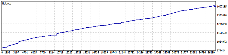
Test on Netting account, 40% profit since 2015 (ratio optimization was carried out over the last year). The drawdown in figures is 0.82%, and the monthly profit is more than 4%. But it is better to launch such a machine without leverage – let it cut profits at a rate slightly better than bonds and USD deposits. Separately,during the test, 7800 lots were traded. This is an additional one and a half percent of profitability in the least.
Overall, I think the idea of transferring the ratios is a good one. In the end, the main thing in algorithmic trading is not the complexity of the system, but its reliability and predictability. Sometimes, seven numbers, correctly selected with the help of modern math, are enough for this.
Important! The EA uses DCA position averaging (time averaging, figuratively speaking), so it is very risky. While tests on Netting with some conservative settings show outstanding results, always remember the danger of averaging positions and that such an EA may drain your deposit to zero in one go!
Ideas for improvement
It is deep night now. I am finishing the article, drinking coffee, looking at the charts on the monitor and thinking about how much more can be done with this system. You know, in algorithmic trading it often happens like this: just when it seems like everything is ready, a dozen new ideas for improvement appear.
And you know what is most interesting? All these improvements must work as a single organism. It is not enough to just throw in a bunch of cool features - they need to complement each other harmoniously, creating a truly reliable trading system.
Ultimately, our goal is not to create a perfect system - it simply does not exist. The goal is to make the system smart enough to make money, but simple enough not to fall apart at the worst possible moment. As the saying goes, the best is the enemy of the good.
| Include | File description |
|---|---|
| MarketSolver.py | Code for selecting ratios and also online trading via Python if necessary |
| MarketSolver.mql5 | MQL5 EA code for trading using selected ratios |
Translated from Russian by MetaQuotes Ltd.
Original article: https://www.mql5.com/ru/articles/16473
Warning: All rights to these materials are reserved by MetaQuotes Ltd. Copying or reprinting of these materials in whole or in part is prohibited.
This article was written by a user of the site and reflects their personal views. MetaQuotes Ltd is not responsible for the accuracy of the information presented, nor for any consequences resulting from the use of the solutions, strategies or recommendations described.

 From Basic to Intermediate: Union (II)
- Free trading apps
- Over 8,000 signals for copying
- Economic news for exploring financial markets
You agree to website policy and terms of use
There are no omissions in the posted Expert Advisor. This is obviously not a code from a real account, there are no filters mentioned here.
Just a demonstration of the idea, which is not bad either.
I agree
Just kapets (sorry)! During several hours of studying your materials for the 10th time I see that we walk the same roads (thoughts).
I really hope that your formulas will help me to formalise mathematically what I already see/use. It will happen only in one case - if I understand them. My mum used to say, "Study, son." I cry bitter tears in maths. I see that many things are simple, but I don't know HOW. I'm trying to get into parabolas, regressions, deviations.... It's hard to go to 6th grade at 65.
// It is not enough to just throw a bunch of cool features - you need them to complement each other harmoniously, creating a really reliable trading system.
Yes. Both the selection of features and the subsequent optimisation are like straightening the figure eight of a bicycle wheel. Some spokes should be loosened, others should be tightened and it should be done in strict obedience to the laws of this process. Then the wheel will be levelled, but if the wrong approach is taken, if the spokes are tightened in the wrong way, it is possible to make a "ten" out of a normal wheel.
In our business "spokes" should help each other, not pull the blanket on themselves to the detriment of other "spokes".
I don't think it's effective to predict price based only on the last two data points.
Do you agree?
I don't think it's effective to predict price based only on the last two data points.
Wouldn't you agree?