Volumetric neural network analysis as a key to future trends

In an era when all trading is becoming more and more automated, it is useful for us to remember the axioms of traders from the past. One of them claims that volume is the key to everything. Indeed, technical analysis and volume analysis would be useful and very interesting to feed as features into machine learning. Perhaps, with the right interpretation, this will give us a result. In this article, we will evaluate the approach to analyzing trading volume and volume-based features using LSTM architecture.

Our system will analyze volume anomalies and predict future price movements. The key features of the system I would like to note are the detection of abnormal volume, volume clustering, and model training directly via the Python + MetaTrader 5 bundle.

We will also conduct comprehensive backtesting with visualization of results. The model demonstrates particular efficiency on the hourly timeframe of the Russian stock market, which is confirmed by the results of testing on historical data of Sberbank shares over the past year. In this article, I will examine in detail the architecture of the system, the principles of its operation and the practical results of its application.

Code breakdown: From data to predictions

Let's dig deep and try to create a system that will really understand what is happening with volumes now. Let's start with simple things - the way we receive and handle data. On the one hand, there is nothing complicated - download the data and work... But the devil, as always, is in the details.

Data source: digging deeper

Below is our data loading function.

def get_mt5_data(self, symbol, timeframe, start_date, end_date):
    try:
        self.logger.info(f"MT5 data request: {symbol}, {timeframe}, {start_date} - {end_date}")
        rates = mt5.copy_rates_range(symbol, timeframe, start_date, end_date)
        df = pd.DataFrame(rates)

It seems pretty simple. I deliberately use copy_rates_range instead of the easier copy_rates_from. We need this so as not to lose zero periods when working with illiquid instruments.

Further on, we begin to work with features and indicators. 

Preprocessing: The art of data preparation

Let's not waste time choosing the features, but instead focus on a few of the most obvious ones. 

def preprocess_data(self, df):
    # Basic volume indicators
    df['vol_ma5'] = df['real_volume'].rolling(window=5).mean()
    df['vol_ma20'] = df['real_volume'].rolling(window=20).mean()
    df['vol_ratio'] = df['real_volume'] / df['vol_ma20']
    
    # ML indicators
    df['price_momentum'] = df['close'].pct_change(24)
    df['volume_momentum'] = df['real_volume'].pct_change(24)
    df['volume_volatility'] = df['real_volume'].pct_change().rolling(24).std()
    df['price_volume_correlation'] = df['price_change'].rolling(24).corr(
        df['real_volume'].pct_change()
    )

Handling feature selection is like tuning an orchestra. Each feature has its own role and its own specific sound in the data symphony. Let's look at our basic set.

The first is the simplest: we take a moving average of volume. The average volume with the period of 5 catches the slightest fluctuations, while the period of 20 reacts to much more powerful volume trends.

The ratio of the volume to its average might also be interesting. When there is a sharp jump in the future, a powerful price impulse very often occurs. 

We also look at price momentum and volume momentum over the last 24 bars.

There is an even more interesting feature called volume volatility. I would call this thing an indicator of market nerves. When volume volatility increases, this may indicate powerful infusions into the market from serious players.

The correlation of price and volume is also considered by our model. At the end, we will definitely look at all these signs live, visualizing our newly-made indicators.

Performance bottleneck

To avoid overloading the system, we can implement data batching and parallel computing. In other words, we divide the data into small pieces and handle them in parallel.

This simple technique speeds up data handling several times, and also helps to avoid problems with memory leaks on large volumes of data. 

In the next part of the article, I will talk about the most interesting part - how the system detects abnormal volumes and what happens next.

In search of "black swans": How to recognize anomalous volumes?

We have all heard about what abnormal volumes are and how to see them on a chart. Perhaps, any experienced trader can spot them. But how can we embed this experience into the code? How to formalize the logic of searching for such volumes? 

Hunting for anomalies

After a series of experiments, my research in this area settled on the Isolation Forest method. Why this method? Well, classical methods like z-scores or percentile scores can miss a local anomaly, a small one, but what is important is not the absolute or percentage values, but the volumes that stand out from the rest - and are out of the general context.

def detect_volume_anomalies(self, df):
    scaler = StandardScaler()
    volume_normalized = scaler.fit_transform(df[['real_volume']])
    
    iso_forest = IsolationForest(contamination=0.1, random_state=42)
    df['is_anomaly'] = iso_forest.fit_predict(volume_normalized)

Of course, it would be better to play around with the parameter, and an even better solution would be to select all the model settings using algorithms like BGA. I set the value to the 0.05 recommended in textbooks, which corresponds to 5% anomalies. But the real market is much noisier than one might imagine. Therefore, the bar has been raised a little. It will also be useful to see the anomalies with your own eyes, in grouping with price movements (we will return to this topic below).

Clustering: Finding patterns

Anomalies are not sufficient for good forecasting. We also need clustering of volumes. We will focus on the following clustering option:

def cluster_volumes(self, df, n_clusters=3):
    features = ['real_volume', 'vol_ratio', 'volatility']
    X = StandardScaler().fit_transform(df[features])
    
    kmeans = KMeans(n_clusters=n_clusters, random_state=42)
    df['volume_cluster'] = kmeans.fit_predict(X)

The features chosen for clustering are quite simple. I think it would be strange to cluster only the actual volumes themselves, otherwise why would we create our features and indicators? However, the number of features, as well as volume indicators, could be improved. 

Three clusters were chosen because I would conditionally divide all volumes into "background or accumulation" volumes, "run and movement" volumes, and "extreme movement" volumes. 

Unexpected finds

Handling the data yielded several patterns and sequences, for example, abnormal volumes are followed by the third cluster of volumes, then goes active volume, and only after that does the quotes move in one direction or another.

This is especially evident in the first hours after the opening of the stock exchange session. It would be useful here to create a heat map of the clusters and their accompanying price movements.

Neural network: How to train a machine to read the market

Since I have been using neural networks for a long time, it would be reasonable to apply a neural network to our volume analysis. I have not tried LSTM architecture yet, but I finally decided to try it after seeing examples of this architecture in other areas.

Let's take a closer look at it. 

Architecture: Less is more

Simpler is better. I came up with a surprisingly simple architecture:

class LSTMModel(nn.Module):
    def __init__(self, input_size, hidden_size=64, num_layers=2, dropout=0.2):
        super(LSTMModel, self).__init__()
        self.lstm = nn.LSTM(
            input_size=input_size,
            hidden_size=hidden_size,
            num_layers=num_layers,
            dropout=dropout,
            batch_first=True
        )
        self.dropout = nn.Dropout(dropout)
        self.linear = nn.Linear(hidden_size, 1)

At first glance, the whole architecture looks very primitive, just two LTSM layers and one linear layer. But the power lies in simplicity. Because, unfortunately, if we build a more extensive network with deeper learning, we will get overfitting. Initially, I built a much more complex network - with three LSTM layers, additional fully connected layers and a complex dropout structure. The results were impressive... On test data. But as soon as the network encountered the real long-term market, everything fell apart. That is, we observed overfitting.

Battle against overfitting

Overfitting is the biggest problem with modern neural networks. The neural network is great at learning to find relationships in test data areas, but is completely lost in real market conditions. Here is how I try to solve this problem specifically in the presented architecture: 

• A single layer cannot handle the complexity of the relationship between volume and price
• Three layers can find connections where they actually do not exist

The size of the hidden layer is chosen in the standard way - 64 neurons. It might be better to use more neurons. In the future, when I introduce a working solution to combat overfitting, we will be able to use a more complex architecture with more neurons.

Input data: The art of feature selection

Let's look at the input features for training:

features = [

    'vol_ratio', 'vol_ma5', 'volatility', 'volume_cluster', 'is_anomaly',

    'price_momentum', 'volume_momentum', 'volume_volatility',

    'price_volume_correlation'

]

We can experiment a lot with the set of features. We can add technical indicators, price derivatives, volume derivatives, price and volume derivatives, whatever we like. But remember that more features will not always improve the quality of forecasting. And every seemingly most logical feature may in fact turn out to be just simple noise in the data.

The combination of 'volume_cluster' and 'is_anomaly' looks interesting here. Individually, the features are modest, but in synergy they are very interesting. When abnormal volumes appear in certain clusters, it has an unusual effect on forecasting. 

Unexpected discovery

The system turned out to be most effective during those periods when price movements are powerful. It also shows itself well in moments that most traders would call unreadable, that is, in sideways markets and during consolidations. It is at these moments that the system for analyzing anomalies and volume clusters sees what is inaccessible to our vision. 

In the next section, I will talk about how this system performed in real trading and share specific examples of signals.  

From forecasts to trading: Turning signals into profits

Any algorithmic trader knows: a simple forecast model is not sufficient. It needs to be developed into a working trading strategy. But how do we apply our model in practice? Let's figure this out. In the next part of the article, you will find not just dry theory, but real practice, with real test trading, strengthening the algorithm, improving the battle against overfitting, but for now, we will get by with the usual theoretical part of our research.

Trading signal anatomy

When developing a trading strategy, one of the key points is the generation of trading signals. In my strategy, signals are generated based on model predictions that reflect the expected return for the next period.

def backtest_prediction_strategy(self, df, lookback=24):
    # Generating signals based on predictions
    df['signal'] = 0
    signal_threshold = 0.001  # Threshold 0.1%
    df.loc[df['predicted_return'] > signal_threshold, 'signal'] = 1
    df.loc[df['predicted_return'] < -signal_threshold, 'signal'] = -1

Selecting the signal threshold

On the one hand, we can set the threshold simply above 0. In this case, we will generate many signals, but they will be noisy due to spread, commissions and market noise. This approach can lead to a large number of false signals, which will negatively affect the strategy efficiency.

Therefore, the most reasonable decision seems to be to raise the threshold of predicted profitability to 0.1%-0.2%. This allows us to cut out most of the noise and reduce the impact of commissions, since signals will only be generated when there are significant predicted price changes.

signal_threshold = 0.001  # Threshold 0.1%

Applying signals considering the shift

Once signals are generated, they are applied to prices taking into account a 24 period forward shift. This allows us to take into account the lag between making a trading decision and its implementation.

df['strategy_returns'] = df['signal'].shift(24) * df['price_change']

A shift of 24 periods means that the signal, generated at the moment t , is applied to the price at the time t + 24. This is important because in reality trading decisions cannot be implemented instantly. This approach allows for a more realistic assessment of the trading strategy efficiency.

Calculating the strategy profitability

The strategy profitability is calculated as the product of the shifted signal and the price change:

df['strategy_returns'] = df['signal'].shift(24) * df['price_change']

If the signal is equal to 1, the strategy profitability will be equal to the price change (price_change). If the signal is equal to -1, the strategy profitability will be equal to the negative price change (-price_change). If the signal is equal to 0, the strategy profitability will be zero.

Thus, shifting signals by 24 periods allows us to take into account the lag between making a trading decision and its implementation, which makes the assessment of the strategy efficiency more realistic.

Golden mean

After weeks of testing, I settled on a threshold of 0.1%. Here is why:

• At this threshold, the system generates signals quite frequently
• About 52-63% of deals are profitable
• The average profit per deal is approximately 2.5 times the commission

The most unusual discovery is that most false signals can also be concentrated in time clusters. If you want, you can consider such a time filter, and we will consider it later, in the next part of the article.

def apply_time_filter(self, df):
    # We trade only during active hours
    trading_hours = df['time'].dt.hour
    df.loc[~trading_hours.between(10, 12), 'signal'] = 0

Risk Management

The logic of position acquisition and the logic of managing open deals (supporting deals during trading) constitutes a separate story. On the one hand, the most obvious solution here is to use fixed stops and takes, but the market is too unpredictable and dynamic for loss and profit limits to be described by ordinary formal logic.  

Our solution is quite trivial - use the predicted volatility to dynamically set stops:

def calculate_stop_levels(self, predicted_return, predicted_volatility):
    base_stop = abs(predicted_return) * 0.7
    volatility_adjust = predicted_volatility * 1.5
    return max(base_stop, volatility_adjust)

This approach also needs to be tested further. It is also possible to apply the VaR risk analysis model to select stops and takes according to this old, but reliably effective system.

Unexpected finds

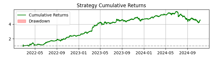
An interesting finding is that series of consecutive signals can predict very strong moves. Issues also arise when the market volatility on average soars very strongly, then our threshold is no longer sufficient for effective trading. If you notice, the periods of drawdowns on the chart are precisely associated with high volatility... But for us, this is not a problem! We will solve and eliminate this problem in the next section.

Visualization and logging: How to avoid drowning in data

It is also very important for us not to forget about the logging system. In general, everything related to prints, logs, outputs and program comments is vital at the debugging stage. This way you can find the source of problems in your code very quickly and efficiently.

Logging system: Details matter

The logging system is based on a simple but efficient format:

log_format = '%(asctime)s [%(levelname)s] %(message)s'
date_format = '%Y-%m-%d %H:%M:%S'

logger = logging.getLogger('VolumeAnalyzer')
logger.setLevel(logging.DEBUG)

What is so difficult about it, you might ask. I discovered this format after several painful experiences when I could not understand why the system opened a position at a particular moment.

Now every action of the system leaves a clear trace in the logs. I also make sure to log the moments related to abnormal volumes:

self.logger.info(f"Abnormal volume detected: {volume:.2f}")
self.logger.debug(f"Context: cluster {cluster}, volatility {volatility:.4f}")

We also need visualization. The experience of manual trading left a strong habit - to observe everything visually, when you look at the data in the same way as you look at the most ordinary chart. Here is our visualization code:

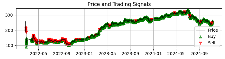
def visualize_results(self, df):
    plt.figure(figsize=(15, 12))
    
    # Price and signal chart
    plt.subplot(3, 1, 1)
    plt.plot(df['time'], df['close'], 'k-', label='Price', alpha=0.7)
    plt.scatter(df[df['signal'] == 1]['time'], 
               df[df['signal'] == 1]['close'],
               marker='^', color='g', label='Buy')

Our first graph is the most common chart of Sber prices with the obtained model signals. We also supplement the signals by highlighting those candles where there are abnormal volumes. This helps us understand the moments when the system reads the market perfectly, like an open book.

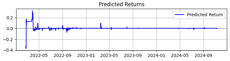
The second graph is the predicted return. Here we can clearly see that before powerful movements of the chosen asset quotes, a very powerful series of forecasts often begins. So this suggests the idea of considering creating a system just on this particular observation. Of course, the number of transactions will fall, but we are not chasing quantity, we are striving for quality, aren’t we?

The third chart is the cumulative return with drawdowns highlighted.

From theory to practice: Results and prospects

Let's sum up the results of the system operation - not just dry numbers, but discoveries that can help everyone interested in volume analysis in trading.

First, the market actually speaks to us through trading turnover and volume. But this language is much more complex than you might imagine. In my personal opinion, classic methods like VSA are rapidly becoming obsolete, failing to keep up with the equally rapid development of the market. Patterns are becoming more complex and volumes form very complicated patterns that are hardly visible to the naked eye.

Overall, as a result of my almost three years of machine learning experience, I can only summarize briefly that the market is becoming more complex every year, and the algorithms that work on it, partly forming trends and accumulations with their OrderFlow, are also becoming more complex. Ahead of us lies the battle of neural networks - the battle of machines for the market determining whose machine will be more efficient.

Summing up the work on the system, I would like to share not only the figures, but also the main discoveries that can be useful to everyone who works with volume analysis.

Over 365 days on SBER shares, the system showed impressive results:

• Total Return: 365.0% per annum (without leverage)
• Share of profitable trades: 50.73%

But these numbers are not the most important thing. More importantly, the system has proven to be resilient to a variety of market conditions. It works equally well in both a trend and a sideways movement, although the nature of the signals changes noticeably.

The system behavior during periods of high volatility turned out to be especially interesting. It is precisely when most traders prefer to stay out of the market that the neural network finds the clearest patterns in the volume flow. Perhaps this is because at such moments institutional players leave more obvious "traces" of their actions.

What this project taught me

1. Machine learning in trading is not a magic pill. Success comes only with a deep understanding of the market and careful engineering of features.
2. Simplicity is the key to sustainability. Every time I tried to complicate the model by adding new layers or features, the system became more and more fragile.
3. Volumes need to be analyzed in context. Anomalous volumes or clusters alone mean little. The magic begins when we look at their interaction with other factors.

What's next?

The system continues to evolve. I am currently working on a few improvements:

• Adaptive parameter adjustment depending on the market phase
• Integrating streaming orders for more accurate analysis
• Expansion to other instruments of the Russian market

The source code of the system is available in the attachments. I would welcome suggestions for improvement. It would be especially interesting to hear the experience of those who will try to adapt the system to other tools.

Conclusion

In conclusion, I would like to note that the most valuable discovery of recent months for me has been the adaptation of classical approaches, such as the volumetric analysis we discussed today, to new technologies such as machine learning, neural networks, and big data.

As it turns out, the experience of past generations is alive and kicking. Our task is to digest this experience, distill it, and improve it from the perspective of our generation of traders, using the latest technologies. And of course, we cannot lag behind the modern era: quantum machine learning, quantum algorithms for forecasting prices and volumes, as well as multidimensional features for machine learning are ahead of us. I have already tried to analyze the market on IBM's 20-qubit quantum supercomputer. The results are interesting, I will definitely tell you about them in future articles.