Economic forecasts: Exploring the Python potential

Introduction

Economic forecasting is a rather complex and labor-intensive task. It allows us to analyze possible future movements using past data. By analyzing historical data and current economic indicators, we can speculate on where the economy might be heading. This is a pretty useful skill. With its help, we can make more informed decisions in business, investments, and economic policy.

We will develop this tool using Python and economic data from collecting information to creating predictive models. It will analyze and also make predictions for the future.

Financial markets are a good barometer of the economy. They react to the slightest changes. The result can be either predictable or unexpected. Let's look at examples where readings cause this barometer to fluctuate.

When GDP grows, markets usually react positively. When inflation rises, unrest is usually expected. When unemployment falls, this is usually seen as good news. However, there might be exceptions. Trade balance, interest rates - each indicator affects market sentiment.

As practice shows, markets often react not to the actual result, but to the expectations of the majority of players. "Buy rumors, sell facts" - this old stock market wisdom most accurately reflects the essence of what is happening. Also, the lack of significant changes can cause more volatility in the market than unexpected news.

Economics is a complex system. Everything is interconnected here and one factor influences another. Changes in one parameter may start a chain reaction. Our task is to understand these connections and learn to analyze them. We will look for solutions using the Python tool.

Setting up the environment: Importing the necessary libraries

So, what do we need? First things first - Python. If you do not have it installed yet, go to python.org. Also, do not forget to check the "Add Python to PATH" box during the installation process.

The next step is libraries. Libraries significantly expand the basic capabilities of our tool. We will need:

1. pandas — for handling data.
2. wbdata — for interaction with the World Bank. With the help of this library, we will get the latest economic data.
3. MetaTrader 5 - we will need it to interact directly with the market itself.
4. CatBoostRegressor from catboost — a small hand-crafted AI.
5. train_test_split and mean_squared_error from sklearn — these libraries will help us evaluate how effective our model is.

To install everything you need, open a command prompt and enter:

pip install pandas wbdata MetaTrader5 catboost scikit-learn

Is everything set? Excellent! Now let's write our first strings of code:

import pandas as pd
import wbdata
import MetaTrader5 as mt5
from catboost import CatBoostRegressor
from sklearn.model_selection import train_test_split
from sklearn.metrics import mean_squared_error
import warnings

warnings.filterwarnings("ignore", category=UserWarning, module="wbdata")

We have prepared all the necessary tools. Let's move on.

Working with the World Bank API: Loading economic indicators

Now let's figure out how we will receive economic data from the World Bank.

First we create a dictionary with indicator codes:

indicators = {
    'NY.GDP.MKTP.KD.ZG': 'GDP growth',  # GDP growth
    'FP.CPI.TOTL.ZG': 'Inflation',      # Inflation
    'FR.INR.RINR': 'Real interest rate', # Real interest rate
    # ... and a bunch of other smart parameters
}

Each of these codes provides access to a specific type of data.

Let's go on. We start a loop that will go through the entire code:

data_frames = []
for indicator in indicators.keys():
    try:
        data_frame = wbdata.get_dataframe({indicator: indicators[indicator]}, country='all')
        data_frames.append(data_frame)
    except Exception as e:
        print(f"Error fetching data for indicator '{indicator}': {e}")

Here we try to get data for each indicator. If it works, we put it on the list. If failed, print an error and move on.

After that, we collect all our data into one big DataFrame:

data = pd.concat(data_frames, axis=1)

At this stage, we need to get all the economic data.

The next step is to save everything we have received to a file so that we can later use it for the purposes we need:

data.to_csv('economic_data.csv', index=True)

We have just downloaded a bunch of data from the World Bank. It is that easy.

Overview of key economic indicators for analysis

If you are a novice, it may be a little difficult to understand a lot of data and numbers. Let's look at the main indicators to make the process easier:

1. GDP growth is a kind of income for a country. Growing indicators are positive, while falling ones have a negative impact on the country.
2. Inflation is the rise in price of goods and services.
3. Real interest rate - if it rises, it makes loans more expensive.
4. Export and import show what a country sells and buys. Higher sales are seen as a positive development.
5. Current account balance - how much money other countries owe to a certain country. Higher numbers indicate good financial condition of a country.
6. Government debt represents the loans of a country. The smaller the numbers, the better.
7. Unemployment - how many people are out of work. Less is better.
8. GDP per capita growth shows whether an average person is getting richer or not.

This looks as follows in the code:

# Loading data from the World Bank
indicators = {
    'NY.GDP.MKTP.KD.ZG': 'GDP growth',  # GDP growth
    'FP.CPI.TOTL.ZG': 'Inflation',       # Inflation
    'FR.INR.RINR': 'Real interest rate', # Real interest rate
    'NE.EXP.GNFS.ZS': 'Exports',         # Exports of goods and services (% of GDP)
    'NE.IMP.GNFS.ZS': 'Imports',         # Imports of goods and services (% of GDP)
    'BN.CAB.XOKA.GD.ZS': 'Current account balance', # Current account balance (% of GDP)
    'GC.DOD.TOTL.GD.ZS': 'Government debt', # Government debt (% of GDP)
    'SL.UEM.TOTL.ZS': 'Unemployment rate', # Unemployment rate (% of total labor force)
    'NY.GNP.PCAP.CD': 'GNI per capita',   # GNI per capita (current US$)
    'NY.GDP.PCAP.KD.ZG': 'GDP per capita growth', # GDP per capita growth (constant 2010 US$)
    'NE.RSB.GNFS.ZS': 'Reserves in months of imports', # Reserves in months of imports
    'NY.GDP.DEFL.KD.ZG': 'GDP deflator', # GDP deflator (constant 2010 US$)
    'NY.GDP.PCAP.KD': 'GDP per capita (constant 2015 US$)', # GDP per capita (constant 2015 US$)
    'NY.GDP.PCAP.PP.CD': 'GDP per capita, PPP (current international $)', # GDP per capita, PPP (current international $)
    'NY.GDP.PCAP.PP.KD': 'GDP per capita, PPP (constant 2017 international $)', # GDP per capita, PPP (constant 2017 international $)
    'NY.GDP.PCAP.CN': 'GDP per capita (current LCU)', # GDP per capita (current LCU)
    'NY.GDP.PCAP.KN': 'GDP per capita (constant LCU)', # GDP per capita (constant LCU)
    'NY.GDP.PCAP.CD': 'GDP per capita (current US$)', # GDP per capita (current US$)
    'NY.GDP.PCAP.KD': 'GDP per capita (constant 2010 US$)', # GDP per capita (constant 2010 US$)
    'NY.GDP.PCAP.KD.ZG': 'GDP per capita growth (annual %)', # GDP per capita growth (annual %)
    'NY.GDP.PCAP.KN.ZG': 'GDP per capita growth (constant LCU)', # GDP per capita growth (constant LCU)
}

Each indicator has its own importance. Individually, they say little, but together they give a more complete picture. It should also be noted that the indicators influence each other. For example, low unemployment is usually good news, but it can lead to higher inflation. Or high GDP growth may not be so positive if it is achieved at the expense of huge debts.

That is why we use machine learning, as it helps us take into account all these complex relationships. It significantly speeds up the process of information processing and sorts data. However, you will also need to put some effort to understand the process.

Handling and structuring World Bank data

Of course, at first glance, the World Bank's wealth of data can seem like a daunting task to understand. To make work and analysis easier, we will collect the data in a table.

data_frames = []
for indicator in indicators.keys():
    try:
        data_frame = wbdata.get_dataframe({indicator: indicators[indicator]}, country='all')
        data_frames.append(data_frame)
    except Exception as e:
        print(f"Error fetching data for indicator '{indicator}': {e}")

data = pd.concat(data_frames, axis=1)

Next, we take each indicator and try to get data for it. There may be problems with individual indicators, we write about it and move on. Then we collect individual data into one large DataFrame.

But we do not stop there. Now the most interesting part begins.

print("Available indicators and their data:")
print(data.columns)
print(data.head())

data.to_csv('economic_data.csv', index=True)

print("Economic Data Statistics:")
print(data.describe())

We look at what we have achieved. What indicators are there? What do the first rows of data look like? It is like the first look at a completed puzzle: is everything in place? And then we save all this stuff into a CSV file. 

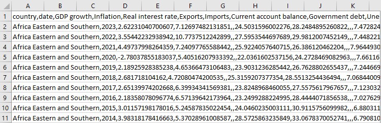
And finally, some statistics. Average values, highs, lows. It is like a quick check - is everything okay with our data? This is how we transform a bunch of disparate numbers into a coherent data system. We now have all the tools for serious economic analysis. 

Introduction to MetaTrader 5: Establishing a connection and receiving data

Now let's talk about MetaTrader 5. First we need to establish a connection. This is what it looks like:

if not mt5.initialize():
    print("initialize() failed")
    mt5.shutdown()

The next important step is getting the data. First, we need to check what currency pairs are available:

symbols = mt5.symbols_get()
symbol_names = [symbol.name for symbol in symbols]

Once the above code is executed, we will get a list of all available currency pairs. Next, we need to download historical quote data for each available pair:

historical_data = {}
for symbol in symbol_names:
    rates = mt5.copy_rates_from_pos(symbol, mt5.TIMEFRAME_D1, 0, 1000)
    df = pd.DataFrame(rates)
    df['time'] = pd.to_datetime(df['time'], unit='s')
    df.set_index('time', inplace=True)
    historical_data[symbol] = df

What is going on in this code we entered? We instructed MetaTrader to download data for the last 1000 days for each trading instrument. After this, the data is loaded into the table.

The downloaded data contains everything that has happened in the currency market over the past three years, in great detail. Now, the received quotes can be analyzed and patterns can be found. The possibilities here are practically unlimited.

Data preparation: Combining economic indicators and market data

At this stage, we will deal directly with data handling. We have two separate sectors: the world of economic indicators and the world of exchange rates. Our task is to bring these sectors together.

Let's start with our data preparation function. This code will be as follows in our general task:

def prepare_data(symbol_data, economic_data):
    data = symbol_data.copy()
    data['close_diff'] = data['close'].diff()
    data['close_corr'] = data['close'].rolling(window=30).corr(data['close'].shift(1))

    for indicator in indicators.keys():
        if indicator in economic_data.columns:
            data[indicator] = economic_data[indicator]
        else:
            print(f"Warning: Data for indicator '{indicator}' is not available.")

    data.dropna(inplace=True)
    return data

Now let's take this step by step. First, we create a copy of the currency pair data. Why? It is always better to work with a copy of data rather than the original. In case of an error, we will not have to create the original file again.

Now comes the most interesting part. We add two new columns: 'close_diff' and 'close_corr'. The first one shows how much the closing price has changed compared to the previous day. This way we will know whether there is a positive or negative shift in price. The second one is the correlation of the closing price with itself, but with a shift of one day. What is this for? In fact, it is simply the most convenient way to understand how similar today's price is to yesterday's one.

Now comes the hard part: we try to add economic indicators to our currency data. This is how we begin to integrate our data into one construct. We go through all our economic indicators and try to find them in the World Bank data. If we find it, great, we add it to our currency data. If not, well, it happens. We just write a warning and move on. 

After all this, we may be left with rows of missing data. We just delete them.

Now let's see how we apply this function:

prepared_data = {}
for symbol, df in historical_data.items():
    prepared_data[symbol] = prepare_data(df, data)

We take each currency pair and apply our written function to it. At the output, we get a ready-made data set for each pair. There will be a separate set for each pair, but they are all assembled according to the same principle.

Do you know what the most important thing in this process is? We are creating something new. We take different economic data and live exchange rate data and create something coherent out of it. Individually they may appear chaotic, but when put together we can identify patterns.

And now we have a ready-made data set for analysis. We can look for sequences in it, make predictions, and draw conclusions. However, we will need to identify the signs that are truly worthy of attention. In the world of data, there are no unimportant details. Every step in data preparation can be critical for the final result.

Machine learning in our model

Machine learning is a rather complex and labor-intensive process. CatBoost Regressor — this function will play an important role later. Here is how we use it:

from catboost import CatBoostRegressor

model = CatBoostRegressor(iterations=1000, learning_rate=0.1, depth=8, loss_function='RMSE', verbose=100)
model.fit(X_train, y_train, verbose=False)

Every parameter is important here. 1000 iterations is how many times the model will run through the data. Learning rate 0.1 - no need to set a high speed right away, we should learn gradually. Depth 8 - looking for complex connections. RMSE — this is how we evaluate errors. Training a model takes a certain amount of time. We show examples and evaluate correct answers. CatBoost works especially well with different types of data. It is not limited to a narrow range of functions.

To forecast currencies, we do the following:

def forecast(symbol_data):
    X = symbol_data.drop(columns=['close'])
    y = symbol_data['close']

    X_train, X_test, y_train, y_test = train_test_split(X, y, test_size=0.5, shuffle=False)

    model = CatBoostRegressor(iterations=1000, learning_rate=0.1, depth=8, loss_function='RMSE', verbose=100)
    model.fit(X_train, y_train, verbose=False)

    predictions = model.predict(X_test)
    mse = mean_squared_error(y_test, predictions)
    print(f"Mean Squared Error for {symbol}: {mse}")

One part of the data is for training, the other is for testing. It is like going to school: first you study, then you take an exam

We divide the data into two parts. Why? One part for training, the other for testing. After all, we will need to test the model on data it has not worked with yet.

After training, the model tries to predict. The root mean square error shows how well it worked. The smaller the error, the better the forecast. CatBoost is notable for the fact that it is constantly improving. It learns from mistakes.

Of course, CatBoost is not an automatic program. It needs good data. Otherwise, we get ineffective data at the input, ineffective data at the output. But with the right data, the result is positive. Now let's talk about data division. I mentioned that we need quotes for verification. Here's how it looks in the code:

X_train, X_test, y_train, y_test = train_test_split(X, y, test_size=0.5, shuffle=False)

50% of the data goes to testing. Do not mix them up - it is important to maintain the time order for the financial data.

Creating and training the model is the most interesting part. Here CatBoost demonstrates its capabilities to the fullest:

model = CatBoostRegressor(iterations=1000, learning_rate=0.1, depth=8, loss_function='RMSE', verbose=100)
model.fit(X_train, y_train, verbose=False)

The model greedily absorbs data looking for patterns. Each iteration is a step towards a better understanding of the market.

And now the moment of truth. Accuracy evaluation:

predictions = model.predict(X_test)
mse = mean_squared_error(y_test, predictions)

The root mean square error is also an important point in our work. It shows how wrong the model is. Less is better. This allows us to evaluate the quality of the program. Remember, there are no final guarantees in trading. But with CatBoost the process is more efficient. It sees things we might miss. And with each forecast the result improves.

Forecasting future values of currency pairs

Forecasting currency pairs is working with probabilities. Sometimes we get positive results, and sometimes we suffer losses. The main thing is that the final result meets our expectations.

In our code, the 'forecast' function works with probabilities. Here is how it performs the calculations:

def forecast(symbol_data):
    X = symbol_data.drop(columns=['close'])
    y = symbol_data['close']

    X_train, X_test, y_train, y_test = train_test_split(X, y, test_size=0.2, shuffle=False)

    model = CatBoostRegressor(iterations=1000, learning_rate=0.1, depth=8, loss_function='RMSE', verbose=100)
    model.fit(X_train, y_train, verbose=False)

    predictions = model.predict(X_test)
    mse = mean_squared_error(y_test, predictions)
    print(f"Mean Squared Error for {symbol}: {mse}")

    future_data = symbol_data.tail(30).copy()
    if len(predictions) >= 30:
        future_data['close'] = predictions[-30:]
    else:
        future_data['close'] = predictions

    future_predictions = model.predict(future_data.drop(columns=['close']))

    return future_predictions

First, we separate the already available data from the predicted data. Then we divide the data into two parts: for training and for testing. The model learns from one set of data, and we test it on another. After training, the model makes predictions. We look at how wrong it was using the root mean square error. The lower the number, the better the forecast.

But the most interesting thing is the analysis of quotes for possible future price movements. We take the last 30 days of data and ask the model to predict what will happen next. It looks like a situation where we resort to the forecasts of experienced analysts. As for visualization... Unfortunately, the code does not yet provide any explicit visualization of the results. But let's add it and see what it might look like:

import matplotlib.pyplot as plt

for symbol, forecast in forecasts.items():
    plt.figure(figsize=(12, 6))
    plt.plot(range(len(forecast)), forecast, label='Forecast')
    plt.title(f'Forecast for {symbol}')
    plt.xlabel('Days')
    plt.ylabel('Price')
    plt.legend()
    plt.savefig(f'{symbol}_forecast.png')
    plt.close()

This code would create a chart for each currency pair. Visually, it is built linearly. Each point is a predicted price for a specific day. These charts are designed to show possible trends, work has been done with a huge array of data, often too complex for the average person. If the line is directed upward, the currency will become more expensive. Falling down? Prepare for a rate decline.

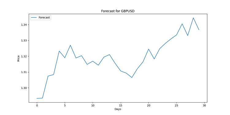
Remember, forecasts are not guarantees. The market may make its own changes. But with good visualization, you will at least know what to expect. After all, in this situation we have a high-quality analysis at our fingertips.

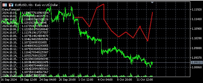
I also made a code to visualize the forecast results in MQL5 by opening a file and outputting forecasts to Comment:

//+------------------------------------------------------------------+
//|                                                 Economic Forecast|
//|                                Copyright 2024, Evgeniy Koshtenko |
//|                          https://www.mql5.com/en/users/koshtenko |
//+------------------------------------------------------------------+
#property copyright "Copyright 2023, Evgeniy Koshtenko"
#property link      "https://www.mql5.com/en/users/koshtenko"
#property version   "4.00"

#property strict
#property indicator_chart_window
#property indicator_buffers 1
#property indicator_plots   1
#property indicator_label1  "Forecast"
#property indicator_type1   DRAW_SECTION
#property indicator_color1  clrRed
#property indicator_style1  STYLE_SOLID
#property indicator_width1  2

double ForecastBuffer[];
input string FileName = "EURUSD_forecast.csv"; // Forecast file name

//+------------------------------------------------------------------+
//| Custom indicator initialization function                         |
//+------------------------------------------------------------------+
int OnInit()
  {
   SetIndexBuffer(0, ForecastBuffer, INDICATOR_DATA);
   PlotIndexSetDouble(0, PLOT_EMPTY_VALUE, EMPTY_VALUE);
   return(INIT_SUCCEEDED);
  }

//+------------------------------------------------------------------+
//| Draw forecast                                                    |
//+------------------------------------------------------------------+
int OnCalculate(const int rates_total,
                const int prev_calculated,
                const datetime &time[],
                const double &open[],
                const double &high[],
                const double &low[],
                const double &close[],
                const long &tick_volume[],
                const long &volume[],
                const int &spread[])
  {
   static bool first=true;
   string comment = "";

   if(first)
     {
      ArrayInitialize(ForecastBuffer, EMPTY_VALUE);
      ArraySetAsSeries(ForecastBuffer, true);
      int file_handle = FileOpen(FileName, FILE_READ|FILE_CSV|FILE_ANSI);
      if(file_handle != INVALID_HANDLE)
        {
         // Skip the header
         string header = FileReadString(file_handle);
         comment += header + "\n";

         // Read data from file
         while(!FileIsEnding(file_handle))
           {
            string line = FileReadString(file_handle);
            string str_array[];
            StringSplit(line, ',', str_array);
            datetime time=StringToTime(str_array[0]);
            double   price=StringToDouble(str_array[1]);
            PrintFormat("%s  %G", TimeToString(time), price);
            comment += str_array[0] + ",     " + str_array[1] + "\n";

            // Find the corresponding bar on the chart and set the forecast value
            int bar_index = iBarShift(_Symbol, PERIOD_CURRENT, time);
            if(bar_index >= 0 && bar_index < rates_total)
              {
               ForecastBuffer[bar_index] = price;
               PrintFormat("%d  %s   %G", bar_index, TimeToString(time), price);
              }
           }

         FileClose(file_handle);
         first=false;
        }
      else
        {
         comment = "Failed to open file: " + FileName;
        }
      Comment(comment);
     }
   return(rates_total);
  }
//+------------------------------------------------------------------+
//| Indicator deinitialization function                              |
//+------------------------------------------------------------------+
void OnDeinit(const int reason)
  {
   Comment("");
  }
//+------------------------------------------------------------------+
//| Create the arrow                                                 |
//+------------------------------------------------------------------+
bool ArrowCreate(const long              chart_ID=0,           // chart ID
                 const string            name="Arrow",         // arrow name
                 const int               sub_window=0,         // subwindow number
                 datetime                time=0,               // anchor point time
                 double                  price=0,              // anchor point price
                 const uchar             arrow_code=252,       // arrow code
                 const ENUM_ARROW_ANCHOR anchor=ANCHOR_BOTTOM, // anchor point position
                 const color             clr=clrRed,           // arrow color
                 const ENUM_LINE_STYLE   style=STYLE_SOLID,    // border line style
                 const int               width=3,              // arrow size
                 const bool              back=false,           // in the background
                 const bool              selection=true,       // allocate for moving
                 const bool              hidden=true,          // hidden in the list of objects
                 const long              z_order=0)            // mouse click priority
  {
//--- set anchor point coordinates if absent
   ChangeArrowEmptyPoint(time, price);
//--- reset the error value
   ResetLastError();
//--- create an arrow
   if(!ObjectCreate(chart_ID, name, OBJ_ARROW, sub_window, time, price))
     {
      Print(__FUNCTION__,
            ": failed to create an arrow! Error code = ", GetLastError());
      return(false);
     }
//--- set the arrow code
   ObjectSetInteger(chart_ID, name, OBJPROP_ARROWCODE, arrow_code);
//--- set anchor type
   ObjectSetInteger(chart_ID, name, OBJPROP_ANCHOR, anchor);
//--- set the arrow color
   ObjectSetInteger(chart_ID, name, OBJPROP_COLOR, clr);
//--- set the border line style
   ObjectSetInteger(chart_ID, name, OBJPROP_STYLE, style);
//--- set the arrow size
   ObjectSetInteger(chart_ID, name, OBJPROP_WIDTH, width);
//--- display in the foreground (false) or background (true)
   ObjectSetInteger(chart_ID, name, OBJPROP_BACK, back);
//--- enable (true) or disable (false) the mode of moving the arrow by mouse
//--- when creating a graphical object using ObjectCreate function, the object cannot be
//--- highlighted and moved by default. Selection parameter inside this method
//--- is true by default making it possible to highlight and move the object
   ObjectSetInteger(chart_ID, name, OBJPROP_SELECTABLE, selection);
   ObjectSetInteger(chart_ID, name, OBJPROP_SELECTED, selection);
//--- hide (true) or display (false) graphical object name in the object list
   ObjectSetInteger(chart_ID, name, OBJPROP_HIDDEN, hidden);
//--- set the priority for receiving the event of a mouse click on the chart
   ObjectSetInteger(chart_ID, name, OBJPROP_ZORDER, z_order);
//--- successful execution
   return(true);
  }

//+------------------------------------------------------------------+
//| Check anchor point values and set default values                 |
//| for empty ones                                                   |
//+------------------------------------------------------------------+
void ChangeArrowEmptyPoint(datetime &time, double &price)
  {
//--- if the point time is not set, it will be on the current bar
   if(!time)
      time=TimeCurrent();
//--- if the point price is not set, it will have Bid value
   if(!price)
      price=SymbolInfoDouble(Symbol(), SYMBOL_BID);
  }
//+------------------------------------------------------------------+

Here is how the forecast looks in the terminal:

Interpretation of results: Analyzing influence of economic factors on exchange rates

Now let's take a closer look at interpreting the results based on your code. We have collected thousands of disparate facts into organized data that also needs to be analyzed.

Let's start with the fact that we have a bunch of economic indicators - from GDP growth to unemployment. Each factor has its own influence on the market background. Individual indicators have their own impact, but together these data influence the final exchange rates.

Take GDP for example. In the code, it is represented by several indicators:

'NY.GDP.MKTP.KD.ZG': 'GDP growth',
'NY.GDP.PCAP.KD.ZG': 'GDP per capita growth',

GDP growth usually strengthens the currency. Why? Because positive news attracts players looking for an opportunity to invest capital for further growth. Investors are drawn to growing economies, increasing demand for their currencies.

On the contrary, inflation ( 'FP.CPI.TOTL.ZG': 'Inflation' ) is an alarming signal for traders. The higher the inflation, the faster the value of money decreases. High inflation usually weakens a currency, simply because services and goods start to become much more expensive in the country in question.

It is interesting to look at the trade balance:

'NE.EXP.GNFS.ZS': 'Exports',
'NE.IMP.GNFS.ZS': 'Imports',
'BN.CAB.XOKA.GD.ZS': 'Current account balance',

These indicators are like scales. If exports outweigh imports, the country receives more foreign currency, which usually strengthens the national currency.

Now let's see how we analyze this in code. CatBoost Regressor is our main tool. Like an experienced conductor, it hears all the instruments at once and understands how they influence each other.

Here is what you can add to the forecast function to better understand the impact of factors:

def forecast(symbol_data):
    # ......

    feature_importance = model.feature_importances_
    feature_names = X.columns
    importance_df = pd.DataFrame({'feature': feature_names, 'importance': feature_importance})
    importance_df = importance_df.sort_values('importance', ascending=False)
    print(f"Feature Importance for {symbol}:")
    print(importance_df.head(10))  # Top 10 important factors

    return future_predictions

This will show us which factors were most important for the forecast of each currency pair. It may turn out that for EUR the key factor is the ECB rate, while for JPY it is Japan's trade balance. Example of data output:

Interpretation for EURUSD:

    1. Price Trend: The forecast shows a upward trend for the next 30 days.

    2. Volatility: The predicted price movement shows low volatility.

    3. Key Influencing Factor: The most important feature for this forecast is 'low'.

    4. Economic Implications:

       - If GDP growth is a top factor, it suggests strong economic performance is influencing the currency.

       - High importance of inflation rate might indicate monetary policy changes are affecting the currency.

       - If trade balance factors are crucial, international trade dynamics are likely driving currency movements.

    5. Trading Implications:

       - Upward trend suggests potential for long positions.

       - Lower volatility might allow for wider stop-losses.

    6. Risk Assessment:

       - Always consider the model's limitations and potential for unexpected market events.

       - Past performance doesn't guarantee future results.

But remember that there are no easy answers in economics. Sometimes a currency strengthens against all odds, and sometimes it falls for no apparent reason. The market often lives on expectations rather than current reality.

Another important point is the time lag. Changes in the economy are not immediately reflected in the exchange rate. It is like steering a huge ship - you turn the wheel, but the ship does not change course instantly. In the code, we use daily data, but some economic indicators are updated less frequently. This may introduce some error into the forecasts. Ultimately, interpreting results is as much an art as a science. The model is a powerful tool, but decisions are always made by a human being. Use this data wisely and may your predictions be accurate!

Searching for non-obvious patterns in economic data

The foreign exchange market is a huge trading platform. It is not characterized by predictable price movements, but in addition to this, there are special events that increase volatility and liquidity at the moment. These are global events.

In our code, we rely on economic indicators:

indicators = {
    'NY.GDP.MKTP.KD.ZG': 'GDP growth',
    'FP.CPI.TOTL.ZG': 'Inflation',
    # ...
}

But what to do when something unexpected happens? For example, a pandemic or a political crisis?

Some kind of "surprise index" would be useful here. Imagine that we add something like this to our code:

def add_global_event_impact(data, event_date, event_magnitude):
    data['global_event'] = 0
    data.loc[event_date:, 'global_event'] = event_magnitude
    data['global_event_decay'] = data['global_event'].ewm(halflife=30).mean()
    return data

# ---
def prepare_data(symbol_data, economic_data):
    # ... ...
    data = add_global_event_impact(data, '2020-03-11', 0.5)  # 
    return data

This would allow us to take into account sudden global events and their gradual attenuation.

But the most interesting question here is how this affects forecasts. Sometimes, global events can completely turn our expectations upside down. For example, during a crisis, "safe" currencies like USD or CHF can strengthen against economic logic.

At such moments, our model's productivity drops. And here it is important not to panic, but to adapt. Perhaps it is worth temporarily reducing the forecast horizon or adding more weight to recent data?

recent_weight = 2 if data['global_event'].iloc[-1] > 0 else 1
model.fit(X_train, y_train, sample_weight=np.linspace(1, recent_weight, len(X_train)))

Remember: in the world of currencies, as in dancing, the main thing is to be able to adapt to the rhythm. Even if this rhythm sometimes changes in the most unexpected ways!

Hunting for anomalies: How to find non-obvious patterns in economic data

Now let's talk about the most interesting part - finding hidden treasures in our data. It is like being a detective, only instead of evidence we have numbers and charts.

We already use quite a lot of economic indicators in our code. But what if there are some non-obvious connections between them? Let's try to find them!

To begin with, we can look at the correlations between different indicators:

correlation_matrix = data[list(indicators.keys())].corr()
print(correlation_matrix)

However, this is just the beginning. The real magic begins when we start looking for non-linear relationships. For example, it may turn out that a change in GDP does not immediately affect the exchange rate, but with a delay of several months.

Let's add some "shifted" metrics to our data preparation function:

def prepare_data(symbol_data, economic_data):
    # ......
    for indicator in indicators.keys():
        if indicator in economic_data.columns:
            data[indicator] = economic_data[indicator]
            data[f"{indicator}_lag_3"] = economic_data[indicator].shift(3)
            data[f"{indicator}_lag_6"] = economic_data[indicator].shift(6)
    # ...

Now our model will be able to capture dependencies with a delay of 3 and 6 months.

But the most interesting thing is the search for completely non-obvious patterns. For example, it might turn out that the EUR rate is strangely correlated with ice cream sales in the US (that is a joke, but you get the idea).

For such purposes, feature extraction methods can be used, for example, PCA (Principal Component Analysis):

from sklearn.decomposition import PCA

def find_hidden_patterns(data):
    pca = PCA(n_components=5)
    pca_result = pca.fit_transform(data[list(indicators.keys())])
    print("Explained variance ratio:", pca.explained_variance_ratio_)
    return pca_result

pca_features = find_hidden_patterns(data)
data['hidden_pattern_1'] = pca_features[:, 0]
data['hidden_pattern_2'] = pca_features[:, 1]

These "hidden patterns" may be the key to more accurate forecasts.

Do not forget about seasonality either. Some currencies may behave differently depending on the time of year. Add month and day of the week information to your data - you might find something interesting!

data['month'] = data.index.month
data['day_of_week'] = data.index.dayofweek

Remember, in a world of data there is always room for discovery. Be curious, experiment, and who knows, maybe you will find that very pattern that will change the world of trading.

Conclusion: Prospects for economic forecasts in algorithmic trading

We started with a simple idea - can we predict exchange rate movements based on economic data? What did we find out? It turns out that this idea has some merit. But it is not as simple as it seems at first glance.

Our code significantly simplifies the analysis of economic data. We have learned to collect information from all over the world, process it, and even made the computer make predictions. But remember that even the most advanced machine learning model is just a tool. It is a very powerful tool, but still a tool.

We saw how CatBoost Regressor can find complex relationships between economic indicators and exchange rates. This allows us to go beyond human capabilities and significantly reduce the time spent on handling and analyzing data. But even such a great tool cannot predict the future with 100% accuracy.

Why? Because the economics is a process that depends on many factors. Today everyone is watching oil prices, while tomorrow the whole world could be turned upside down by some unexpected event. We mentioned this effect when talking about the "surprise index". That is exactly why it is so important.