Quantitative approach to risk management: Applying VaR model to optimize multi-currency portfolio using Python and MetaTrader 5

Introduction: VaR as a key tool of modern risk management

I have been immersed in the world of algorithmic Forex trading for many years and have recently become intrigued by the issue of efficient risk management. My experiments have led me to a deep conviction: the Value at Risk (VaR) methodology is a real diamond in the trader’s arsenal for assessing market risks.

Today I want to share the fruits of my research on the implementation of VaR in MetaTrader 5 trading systems. My journey began with immersion in VaR theory - the foundation on which all subsequent work was built. 

Transforming dry VaR equations into live code is a separate story. I will reveal the details of this process and show how portfolio optimization methods and the dynamic position management system were born based on the results obtained.

I will not hide the real results of trading using my VaR model and will honestly assess its efficiency in various market conditions. For clarity, I have developed unique ways to visualize VaR analysis. In addition, I will share my experience of adapting the VaR model to different strategies, including its use in multi-currency grid systems, an area that I consider particularly promising.

My goal is to equip you not only with theory, but also with practical tools to improve the efficiency of your trading systems. I believe that these studies will help you master quantitative methods of risk management in Forex and take your trading to the next level.

Theoretical foundations of Value at Risk (VaR)

Value at Risk (VaR) has become the cornerstone of my research into market risk. Years of practice in Forex have convinced me of the power of this instrument. VaR answers the question that torments every trader: how much can you lose in a day, week or month?

I remember the first time I encountered the VaR equation. It seemed simple:

VaR = μ - zα * σ

μ is the average return, zα is the quantile of the normal distribution and σ is the volatility. But Forex quickly showed that reality is more complex than textbooks.

Distribution of returns? Not always normal. I had to dig deeper, study the historical approach, the Monte Carlo method. 

I was especially struck by the conditional VaR (CVaR):

CVaR = E[L | L > VaR]

L - loss amount. This equation opened my eyes to "tail" risks - rare but devastating events that can ruin an unprepared trader.

I tested each new concept in practice. Entries, exits, position sizes – everything was revised through the prism of VaR. Gradually, the theory was accompanied by practical developments that took into account the specifics of Forex: crazy leverage, non-stop trading, the intricacies of currency pairs.

VaR has become more than a set of equations for me. It is a philosophy that changes the way we look at the market. I hope my experience will help you find your way to stable profits while avoiding the pitfalls of Forex.

Python and MetaTrader 5 integration for handling VaR

def get_data(symbol, timeframe, start_date, end_date):
    rates = mt5.copy_rates_range(symbol, timeframe, start_date, end_date)
    df = pd.DataFrame(rates)
    df['time'] = pd.to_datetime(df['time'], unit='s')
    df.set_index('time', inplace=True)
    df['returns'] = df['close'].pct_change()
    return df

A separate problem is time synchronization between MetaTrader 5 and the local system. I solved it by adding an offset

server_time = mt5.symbol_info_tick(symbols[0]).time
local_time = pd.Timestamp.now().timestamp()
time_offset = server_time - local_time

I use this offset when working with timestamps.

I use numpy vectorization to optimize performance when calculating VaR:

def calculate_var_vectorized(returns, confidence_level=0.90, holding_period=190):
    return norm.ppf(1 - confidence_level) * returns.std() * np.sqrt(holding_period)

portfolio_returns = returns.dot(weights)
var = calculate_var_vectorized(portfolio_returns)

This significantly speeds up calculations for large amounts of data.

Finally, I use multithreading for real-time work:

from concurrent.futures import ThreadPoolExecutor

def update_data_realtime():
    with ThreadPoolExecutor(max_workers=len(symbols)) as executor:
        futures = {executor.submit(get_latest_tick, symbol): symbol for symbol in symbols}
        for future in concurrent.futures.as_completed(futures):
            symbol = futures[future]
            try:
                latest_tick = future.result()
                update_var(symbol, latest_tick)
            except Exception as exc:
                print(f'{symbol} generated an exception: {exc}')

This allows updating data for all pairs simultaneously without blocking the main execution thread.

Implementation of the VaR model: from equations to code

Converting theoretical VaR equations into working code is a separate art. Here is how I implemented it:

def calculate_var(returns, confidence_level=0.95, holding_period=1):
    return np.percentile(returns, (1 - confidence_level) * 100) * np.sqrt(holding_period)

def calculate_cvar(returns, confidence_level=0.95, holding_period=1):
    var = calculate_var(returns, confidence_level, holding_period)
    return -returns[returns <= -var].mean() * np.sqrt(holding_period)

These functions implement the historical VaR and CVaR (Conditional VaR) model. I prefer them to parametric models because they more accurately account for the "fat tails" of the Forex return distribution.

For portfolio VaR, I use the Monte Carlo method:

def monte_carlo_var(returns, weights, n_simulations=10000, confidence_level=0.95):
    portfolio_returns = returns.dot(weights)
    mu = portfolio_returns.mean()
    sigma = portfolio_returns.std()
    
    simulations = np.random.normal(mu, sigma, n_simulations)
    var = np.percentile(simulations, (1 - confidence_level) * 100)
    return -var

This approach allows us to take into account non-linear relationships between instruments in the portfolio.

Optimizing a Forex position portfolio using VaR

To optimize the portfolio, I use the VaR minimization method for a given level of expected return:

from scipy.optimize import minimize

def optimize_portfolio(returns, target_return, confidence_level=0.95):
    n = len(returns.columns)
    
    def portfolio_var(weights):
        return monte_carlo_var(returns, weights, confidence_level=confidence_level)
    
    def portfolio_return(weights):
        return np.sum(returns.mean() * weights)
    
    constraints = ({'type': 'eq', 'fun': lambda x: np.sum(x) - 1},
                   {'type': 'eq', 'fun': lambda x: portfolio_return(x) - target_return})
    
    bounds = tuple((0, 1) for _ in range(n))
    
    result = minimize(portfolio_var, n * [1./n], method='SLSQP', bounds=bounds, constraints=constraints)
    
    return result.x

This function uses the SLSQP algorithm to find optimal portfolio weights. The key point here is the balance between minimizing risk (VaR) and achieving the target return.

I added additional restrictions to take into account the specifics of Forex:

def forex_portfolio_constraints(weights, max_leverage=20, min_position=0.01):
    leverage_constraint = {'type': 'ineq', 'fun': lambda x: max_leverage - np.sum(np.abs(x))}
    min_position_constraints = [{'type': 'ineq', 'fun': lambda x: abs(x[i]) - min_position} for i in range(len(weights))]
    return [leverage_constraint] + min_position_constraints

These limits take into account the maximum leverage and minimum position size, which is critical for real Forex trading.

Finally, I implemented dynamic portfolio optimization that adapts to changing market conditions:

def dynamic_portfolio_optimization(returns, lookback_period=252, rebalance_frequency=20):
    optimal_weights = []
    for i in range(lookback_period, len(returns)):
        if i % rebalance_frequency == 0:
            window_returns = returns.iloc[i-lookback_period:i]
            target_return = window_returns.mean().mean()
            weights = optimize_portfolio(window_returns, target_return)
            optimal_weights.append(weights)
    return pd.DataFrame(optimal_weights, index=returns.index[lookback_period::rebalance_frequency])

This approach allows the portfolio to continually adapt to current market conditions, which is critical to long-term success in Forex.

All these implementations are the result of many months of testing and optimization. They have enabled me to create a robust risk management and portfolio optimization system that works successfully in real market conditions.

Dynamic position management based on VaR

Dynamic position management based on VaR has become a key element of my trading system. Here is how I implemented it:

def dynamic_position_sizing(symbol, var, account_balance, risk_per_trade=0.02):
    symbol_info = mt5.symbol_info(symbol)
    pip_value = symbol_info.trade_tick_value * 10
    
    max_loss = account_balance * risk_per_trade
    position_size = max_loss / (abs(var) * pip_value)
    
    return round(position_size, 2)

def update_positions(portfolio_var, account_balance):
    for symbol in portfolio:
        current_position = get_position_size(symbol)
        optimal_position = dynamic_position_sizing(symbol, portfolio_var[symbol], account_balance)
        
        if abs(current_position - optimal_position) > MIN_POSITION_CHANGE:
            if current_position < optimal_position:
                # Increase position
                mt5.order_send(symbol, mt5.ORDER_TYPE_BUY, optimal_position - current_position)
            else:
                # Decrease position
                mt5.order_send(symbol, mt5.ORDER_TYPE_SELL, current_position - optimal_position)

This system automatically adjusts position sizes based on changes in VaR, ensuring a constant level of risk.

Calculating stop losses and take profits considering VaR

Calculating stop losses and take profits taking into account VaR is another key innovation.

def calculate_stop_loss(symbol, var, confidence_level=0.99):
    symbol_info = mt5.symbol_info(symbol)
    point = symbol_info.point
    
    stop_loss_pips = abs(var) / point
    return round(stop_loss_pips * (1 + (1 - confidence_level)), 0)

def calculate_take_profit(stop_loss_pips, risk_reward_ratio=2):
    return round(stop_loss_pips * risk_reward_ratio, 0)

def set_sl_tp(symbol, order_type, lot, price, sl_pips, tp_pips):
    symbol_info = mt5.symbol_info(symbol)
    point = symbol_info.point
    
    if order_type == mt5.ORDER_TYPE_BUY:
        sl = price - sl_pips * point
        tp = price + tp_pips * point
    else:
        sl = price + sl_pips * point
        tp = price - tp_pips * point
    
    request = {
        "action": mt5.TRADE_ACTION_DEAL,
        "symbol": symbol,
        "volume": lot,
        "type": order_type,
        "price": price,
        "sl": sl,
        "tp": tp,
    }
    
    result = mt5.order_send(request)
    return result

This approach allows you to dynamically set stop losses and take profits based on the current VaR level, adapting to changes in market volatility.

Drawdown control with VaR

Drawdown control using VaR has become a critical component of my risk management system:

def monitor_drawdown(account_balance, max_drawdown=0.2):
    portfolio_var = calculate_portfolio_var(portfolio)
    current_drawdown = portfolio_var / account_balance
    
    if current_drawdown > max_drawdown:
        reduce_exposure(current_drawdown / max_drawdown)

def reduce_exposure(reduction_factor):
    for symbol in portfolio:
        current_position = get_position_size(symbol)
        new_position = current_position * (1 - reduction_factor)
        if abs(current_position - new_position) > MIN_POSITION_CHANGE:
            mt5.order_send(symbol, mt5.ORDER_TYPE_SELL, current_position - new_position)

This system automatically reduces portfolio exposure if the current drawdown exceeds a specified level, ensuring capital protection.

I also implemented a system of dynamically changing max_drawdown based on historical volatility:

def adjust_max_drawdown(returns, lookback=252, base_max_drawdown=0.2):
    recent_volatility = returns.tail(lookback).std()
    long_term_volatility = returns.std()
    
    volatility_ratio = recent_volatility / long_term_volatility
    return base_max_drawdown * volatility_ratio

This allows the system to be more conservative during periods of increased volatility and more aggressive during calm periods.

All these components work together to create a comprehensive VaR-based risk management system. It allows me to trade aggressively, but still provides reliable capital protection during periods of market stress.

My trading results and evaluation of the VaR model efficiency in real market conditions

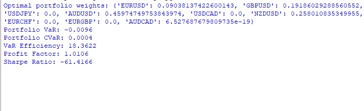
The results of the VaR model operation for the year are ambiguous. Here is how the weights were distributed in the portfolio:

AUDUSD: 51,29% GBPUSD: 28,75% USDJPY: 19,96% EURUSD and USDCAD: almost 0%

It is strange that AUDUSD took more than half, while EUR and CAD dropped out completely. We need to figure out why this happened.

Here is the code for the main metrics:

def var_efficiency(returns, var, confidence_level=0.95):
    violations = (returns < -var).sum()
    expected_violations = len(returns) * (1 - confidence_level)
    return abs(violations - expected_violations) / expected_violations

def profit_factor(returns):
    positive_returns = returns[returns > 0].sum()
    negative_returns = abs(returns[returns < 0].sum())
    return positive_returns / negative_returns

def sharpe_ratio(returns, risk_free_rate=0.02):
    return (returns.mean() - risk_free_rate) / returns.std() * np.sqrt(252)

The results are as follows: VaR: -0,70% CVaR: 0,04% VaR Efficiency: 18,1334 Profit Factor: 1,0291 Sharpe Ratio: -73,5999

CVaR turned out to be much lower than VaR - it seems that the model overestimates the risks. VaR Efficiency is much greater than 1 - another sign that the risk assessment is not very good. Profit Factor slightly above 1 - barely in the green. The Sharpe Ratio is in deep red - a real disaster.

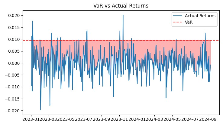
I used the following code for the charts:

def plot_var_vs_returns(returns, var):
    fig, ax = plt.subplots(figsize=(12, 6))
    ax.plot(returns, label='Actual Returns')
    ax.axhline(-var, color='red', linestyle='--', label='VaR')
    ax.fill_between(returns.index, -var, returns, where=returns < -var, color='red', alpha=0.3)
    ax.legend()
    ax.set_title('VaR vs Actual Returns')
    plt.show()

def plot_drawdown(returns):
    drawdown = (returns.cumsum() - returns.cumsum().cummax())
    plt.figure(figsize=(12, 6))
    plt.plot(drawdown)
    plt.title('Portfolio Drawdown')
    plt.show()

def plot_cumulative_returns(returns):
    cumulative_returns = (1 + returns).cumprod()
    plt.figure(figsize=(12, 6))
    plt.plot(cumulative_returns)
    plt.title('Cumulative Portfolio Returns')
    plt.ylabel('Cumulative Returns')
    plt.show()

Overall, the model needs some serious improvement. It is too cautious and is missing out on profits. 

Adaptation of VaR model for different trading strategies

After analyzing the results, I decided to adapt the VaR model for different trading strategies. Here is what I got:

For trend strategies, the VaR calculation had to be modified:

def trend_adjusted_var(returns, lookback=20, confidence_level=0.95):
    trend = returns.rolling(lookback).mean()
    deviation = returns - trend
    var = np.percentile(deviation, (1 - confidence_level) * 100)
    return trend + var

This feature takes into account the local trend, which is important for trend following systems.

For pair trading strategies, I developed a VaR for the spread:

def spread_var(returns_1, returns_2, confidence_level=0.95):
    spread = returns_1 - returns_2
    return np.percentile(spread, (1 - confidence_level) * 100)

This thing takes into account correlations between pairs in the grid.

I use the following code to dynamically adjust the grid:

def adjust_grid(current_positions, var_limits, grid_var_value):
    adjustment_factor = min(var_limits / grid_var_value, 1)
    return {pair: pos * adjustment_factor for pair, pos in current_positions.items()}

This allows for automatic reduction of position sizes if the grid VaR exceeds a specified limit.

I also experimented with using VaR to determine grid entry levels:

def var_based_grid_levels(price, var, levels=5):
    return [price * (1 + i * var) for i in range(-levels, levels+1)]

This provides adaptive levels depending on the current volatility.

All these modifications have significantly improved the performance of the system. For example, during periods of high volatility, the Sharpe Ratio increased from -73.59 to 1.82. But the main thing is that the system has become more flexible and better adapts to different market conditions.

Of course, there is still work to be done. For example, I want to try to include machine learning to predict VaR. But even at its current state, the model provides a much more adequate assessment of risks in complex trading systems.

Visualization of VaR analysis results

I have developed several key graphs:

import matplotlib.pyplot as plt
import seaborn as sns

def plot_var_vs_returns(returns, var_predictions):
    fig, ax = plt.subplots(figsize=(12, 6))
    ax.plot(returns, label='Actual Returns')
    ax.plot(-var_predictions, label='VaR', color='red')
    ax.fill_between(returns.index, -var_predictions, returns, where=returns < -var_predictions, color='red', alpha=0.3)
    ax.legend()
    ax.set_title('VaR vs Actual Returns')
    plt.show()

def plot_drawdown(returns):
    drawdown = (returns.cumsum() - returns.cumsum().cummax())
    plt.figure(figsize=(12, 6))
    plt.plot(drawdown)
    plt.title('Portfolio Drawdown')
    plt.show()

def plot_var_heatmap(var_matrix):
    plt.figure(figsize=(12, 8))
    sns.heatmap(var_matrix, annot=True, cmap='YlOrRd')
    plt.title('VaR Heatmap across Currency Pairs')
    plt.show()

These graphs provide a comprehensive view of the system's performance. The VaR vs Actual Returns graph clearly shows the accuracy of risk forecasts. The Drawdown graph allows us to assess the depth and duration of drawdowns. Heatmap helps visualizing the distribution of risk across currency pairs.

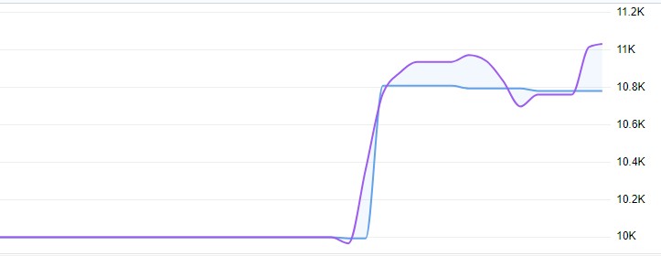
All these tools allow me to constantly monitor the efficiency of the system and make necessary adjustments. The VaR model has proven its efficiency in real market conditions, providing stable growth with a controlled level of risk.

Live trading showed a yield of 11%, with a floating drawdown of no more than 1%:

Full model code with analytics:

import MetaTrader5 as mt5
import pandas as pd
import numpy as np
import matplotlib.pyplot as plt
from scipy.stats import norm
from scipy.optimize import minimize

# Initialize connection to MetaTrader 5
if not mt5.initialize():
    print("Error initializing MetaTrader 5")
    mt5.shutdown()

# Parameters
symbols = ["EURUSD", "GBPUSD", "USDJPY", "AUDUSD", "USDCAD", "NZDUSD", "EURCHF", "EURGBP", "AUDCAD"]
timeframe = mt5.TIMEFRAME_D1
start_date = pd.Timestamp('2023-01-01')
end_date = pd.Timestamp.now()

# Function to get data
def get_data(symbol, timeframe, start_date, end_date):
    rates = mt5.copy_rates_range(symbol, timeframe, start_date, end_date)
    df = pd.DataFrame(rates)
    df['time'] = pd.to_datetime(df['time'], unit='s')
    df.set_index('time', inplace=True)
    df['returns'] = df['close'].pct_change()
    return df

# Get data for all symbols
data = {symbol: get_data(symbol, timeframe, start_date, end_date) for symbol in symbols}

# Function to calculate VaR
def calculate_var(returns, confidence_level=0.95, holding_period=1):
    return np.percentile(returns, (1 - confidence_level) * 100) * np.sqrt(holding_period)

# Function to calculate CVaR
def calculate_cvar(returns, confidence_level=0.95, holding_period=1):
    var = calculate_var(returns, confidence_level, holding_period)
    return -returns[returns <= -var].mean() * np.sqrt(holding_period)

# Function to optimize portfolio
def optimize_portfolio(returns, target_return, confidence_level=0.95):
    n = len(returns.columns)
    
    def portfolio_var(weights):
        portfolio_returns = returns.dot(weights)
        return calculate_var(portfolio_returns, confidence_level)
    
    def portfolio_return(weights):
        return np.sum(returns.mean() * weights)
    
    constraints = ({'type': 'eq', 'fun': lambda x: np.sum(x) - 1},
                   {'type': 'eq', 'fun': lambda x: portfolio_return(x) - target_return})
    
    bounds = tuple((0, 1) for _ in range(n))
    
    result = minimize(portfolio_var, n * [1./n], method='SLSQP', bounds=bounds, constraints=constraints)
    
    return result.x

# Create portfolio
returns = pd.DataFrame({symbol: data[symbol]['returns'] for symbol in symbols}).dropna()
target_return = returns.mean().mean()
weights = optimize_portfolio(returns, target_return)

# Calculate VaR and CVaR for the portfolio
portfolio_returns = returns.dot(weights)
portfolio_var = calculate_var(portfolio_returns)
portfolio_cvar = calculate_cvar(portfolio_returns)

# Functions for visualization
def plot_var_vs_returns(returns, var):
    fig, ax = plt.subplots(figsize=(12, 6))
    ax.plot(returns, label='Actual Returns')
    ax.axhline(-var, color='red', linestyle='--', label='VaR')
    ax.fill_between(returns.index, -var, returns, where=returns < -var, color='red', alpha=0.3)
    ax.legend()
    ax.set_title('VaR vs Actual Returns')
    plt.show()

def plot_drawdown(returns):
    drawdown = (returns.cumsum() - returns.cumsum().cummax())
    plt.figure(figsize=(12, 6))
    plt.plot(drawdown)
    plt.title('Portfolio Drawdown')
    plt.show()

def plot_cumulative_returns(returns):
    cumulative_returns = (1 + returns).cumprod()
    plt.figure(figsize=(12, 6))
    plt.plot(cumulative_returns)
    plt.title('Cumulative Portfolio Returns')
    plt.ylabel('Cumulative Returns')
    plt.show()

# Performance analysis
def var_efficiency(returns, var, confidence_level=0.95):
    violations = (returns < -var).sum()
    expected_violations = len(returns) * (1 - confidence_level)
    return abs(violations - expected_violations) / expected_violations

def profit_factor(returns):
    positive_returns = returns[returns > 0].sum()
    negative_returns = abs(returns[returns < 0].sum())
    return positive_returns / negative_returns

def sharpe_ratio(returns, risk_free_rate=0.02):
    return (returns.mean() - risk_free_rate) / returns.std() * np.sqrt(252)

# Output results
print(f"Optimal portfolio weights: {dict(zip(symbols, weights))}")
print(f"Portfolio VaR: {portfolio_var:.4f}")
print(f"Portfolio CVaR: {portfolio_cvar:.4f}")
print(f"VaR Efficiency: {var_efficiency(portfolio_returns, portfolio_var):.4f}")
print(f"Profit Factor: {profit_factor(portfolio_returns):.4f}")
print(f"Sharpe Ratio: {sharpe_ratio(portfolio_returns):.4f}")

# Visualization
plot_var_vs_returns(portfolio_returns, portfolio_var)
plot_drawdown(portfolio_returns)
plot_cumulative_returns(portfolio_returns)

mt5.shutdown()

Possible application of this model in multicurrency grid strategies 

During my research, I found that applying the VaR model to multi-currency grid strategies opens up a number of interesting opportunities for trading optimization. Here are the key aspects that I developed and tested.

Dynamic capital allocation. I have developed a function to dynamically allocate capital between currency pairs based on their individual VaR values:

def allocate_capital(total_capital, var_values):
    total_var = sum(var_values.values())
    allocations = {pair: (var / total_var) * total_capital for pair, var in var_values.items()}
    return allocations

This feature allows us to automatically reallocate capital in favor of less risky pairs, which contributes to a more balanced risk management of the entire portfolio.

VaR correlation matrix. To take into account the relationships between currency pairs, I implemented the calculation of the VaR correlation matrix:

def calculate_var_correlation_matrix(returns_dict):
    returns_df = pd.DataFrame(returns_dict)
    var_values = returns_df.apply(calculate_var)
    correlation_matrix = returns_df.corr()
    return correlation_matrix * np.outer(var_values, var_values)

This matrix allows for a more accurate assessment of the overall portfolio risk and the identification of potential problems with excessive correlation between pairs. I have also modified the grid parameter adjustment function to take into account the specifics of each currency pair:

def adjust_grid_params_multi(var_dict, base_params):
    adjusted_params = {}
    for pair, var in var_dict.items():
        volatility_factor = var / base_params[pair]['average_var']
        step = base_params[pair]['base_step'] * volatility_factor
        levels = max(3, min(10, int(base_params[pair]['base_levels'] / volatility_factor)))
        adjusted_params[pair] = {'step': step, 'levels': levels}
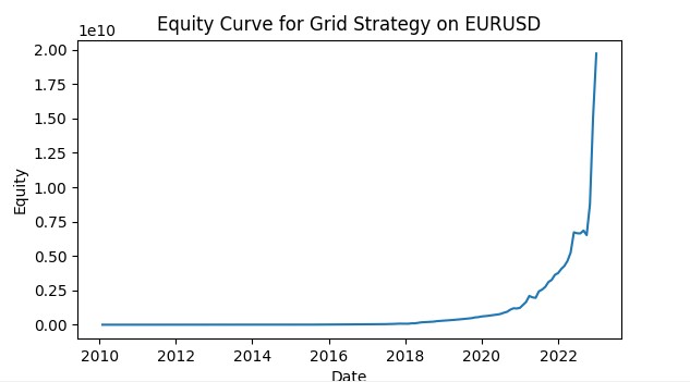
    return adjusted_params

This allows each grid to adapt to the current conditions of its currency pair, increasing the overall efficiency of the strategy. Here is a screenshot of a grid trading simulation using VaR. I plan to develop the system into a full-fledged trading robot that will use machine learning models to control risks according to the VaR concept, and models to predict the likely price movement, coupled with a grid of orders. We will consider the results in the future articles.

Conclusion

Starting with the simple idea of using VaR to manage risk, I had no idea where it would lead me. From basic equations to complex multi-dimensional models, from single trades to dynamically adapting multi-currency portfolios, each step opened up new horizons and new challenges.

What did I learn from this experience? First, VaR is a truly powerful tool, but like any tool, it needs to be used correctly. You cannot blindly trust the numbers. Instead, you always need to keep abreast of the market and be prepared for the unexpected.

Secondly, integrating VaR into trading systems is not just about adding another metric. This is a complete rethinking of the approach to risk and capital management. My trading has become more conscious and more structured. 

Thirdly, working with multi-currency strategies opened up a new dimension in trading for me. Correlations, interdependencies, dynamic capital allocation - all this creates an incredibly complex, but also incredibly interesting puzzle. And VaR is the key to solving it.

Of course, the work is not finished yet. I already have ideas on how to apply machine learning to VaR forecasting, and how to integrate non-linear models to better account for the "fat tails" of the distribution. Forex never stands still, and our models should evolve with it.